VituixCAD
The Loudspeaker Simulation Tool
User Manual
Version 2.0.135.2 (2026-04-25)Copyright © Kimmo Saunisto 2026
kimmo.saunisto@gmail.com
VituixCADThe Loudspeaker Simulation ToolUser ManualVersion 2.0.135.2 (2026-04-25)Copyright © Kimmo Saunisto 2026 kimmo.saunisto@gmail.com |
VituixCAD is loudspeaker simulation software. Design philosophy is to simulate loudspeaker behavior in full space or half space. Even though emphasis is on power response, polar responses and directivity index, it is possible to design a loudspeaker without comprehensive angled measurements. This is not encouraged though.
Software package includes everything one needs for simulating and designing a loudspeaker. Additional to crossover simulator, there is enclosure simulator, diffraction simulator, response tracer, response merger, response calculator, auxiliary calculator and FFT tool included.
Recommended platform is Windows 10 or 11 in real or virtual machine such as VMware (Player 16) or VirtualBox. Could run also on Wine with .NET 4.8 installed, but it's not quaranteed. Performance and features could be radically reduced compared to Windows 10-11 in real machine.
Download the latest build: VituixCAD2_setup.exe. See also changelog.
VituixCAD could run also on Linux, but it's not guaranteed and supported and some functions might be slow.
Installation to Linux with Wine: VituixCAD in Linux v0.3.pdf
Public folders created by setup program:
| \Users\Public\Documents\VituixCAD\Enclosure | Local driver database (VituixCAD_Drivers.txt/.vxd/.xml) |
| \Users\Public\Documents\VituixCAD\Library | Library blocks (.vxl, .png) |
| \Users\Public\Documents\VituixCAD\Projects | Response file samples (.txt) |
| \Users\Public\Documents\VituixCAD\Template | LTspice templates (.asc, .plt) |
User folders created while running if not already exist:
| \Users\username\Documents\VituixCAD\Download | Download folder for auto update |
| \Users\username\Documents\VituixCAD\Enclosure | LTspice files (.asc, .plt, .log, .net, .raw) |
| \Users\username\Documents\VituixCAD\Projects | User projects (.vxp, .vxe, .vxm, .vxb, .txt, .frd, .zma, ...) |
| VituixCAD.exe "path\filename" | Opens VituixCAD project file ending with ".vxp", ".vxe", ".vxb", ".vxf", ".vxm" |
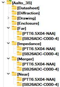
All files included in loudspeaker project should be located to \Users\username\Documents\VituixCAD\Projects\projectname and it's subdirectories in order to help archiving as zip-file and distribution to other users. Project folders can be created with 'Create project subfolders' window integrated to File->New command. Two different hierarchy options are available:

This hierarchy option supports typical measurement sequence: 1) Far field measurements of all drivers 2) Near field measurements of all drivers and ports 3) Impedance measuremenents of all drivers.
Enter driver models to the table and check Common folders and Data folders you want to create.

This hierarchy option locates measurement data of a single driver to the same folder. It could help copying data to different project using the same driver+enclosure -combination.
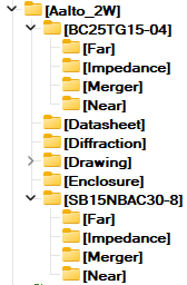
Save all project files .vxp, .vxe, .vxb, .vxm to the main folder of the project (VituixCAD\Projects\projectname).
Typical content of Common folders:
| Datasheet | Datasheets of drivers, connectors, amplifiers and other components. |
| Diffraction | Baffle effect responses for quasi near field to far field conversion with Merger tool. Possible simulated directivity i.e. off-axis responses of sub-...mid-woofers. BEM simulations with Akabak etc. |
| Drawing | 2D and 3D drawings, manufacturing instructions and parts lists. |
| Enclosure | Simulated half space frequency and impedance responses for preliminary studies. |
| Export | Miscellaneous exports such as power dissipation, time domain and transfer functions of FIR filters. |
| Room | Acoustic parameter and in-room response measurements. |
Typical content of Data folders:
| Far | Far field measurements and FR exports: .pir/.mls/.crp/.mdat, .txt/.frd. |
| Impedance | Impedance response measurements and ZR exports: .pir/.mls/.sin/.crp/.mdat, .txt/.zma. |
| Merger | Merged responses: .frd/.txt. |
| Near | Near field measurements and FR exports: .pir/.mls/.crp/.mdat, .txt/.frd. |
Create button creates also empty project (.vxp) with driver models listed to the table.
Press F1 for help.
The latest online manual can also be opened to your default browser from the internet. Add bookmark to the browser for fast access to the latest revision.

This user guide is a chronological walkthrough on how to design a loudspeaker with VituixCAD. Commonly, design process starts with deciding enclosure size, drivers, radiator type, alignment etc. Enclosure tool is used for simulating enclosures, different radiator types and alignments. Next step is to have comprehensive set of acoustic and electrical measurements of the construction. Diffraction and Merger tools are used for combining far field and near field responses. After these prerequisites are met, simulation phase can be started. Whether your goal is to design a speaker with or without interim listening tests, you'll need quality control of some sort. Some prefer their ears, some prefer measurements. If a loudspeaker measures perfectly, but sounds worse than anything you've ever heard, something is terribly wrong. This guide will not teach you how to listen a loudspeaker, but will cover basic QC steps.
Building prototypes and crossovers are not covered in this guide. This guide will also assume you have suitable measurement gear and software and understanding about how to measure loudspeaker drivers for design purposes.
Investigate acoustic parameters, dimensions, materials and speaker placement possibilities of the listening room. It is wise to fix issues of bad environment (the room) first rather than trying to handle everything with massive and complex speaker design.
Export frequency responses with Convert IR to FR tool if measured with CLIO or ARTA, or measurements are exported to wav files. This is not needed with REW 5.20 beta 7 or later having group export.
Mandatory QC-measurements
Additional QC-measurements
Listen to your favorite tracks.
If you are not satisfied return to drawing board.

Main window is divided into two sections, control section on the left and graphs on the right.
| New | Create new empty project |
| Open | Open existing project |
| Recent > | Open previously opened project |
| Save (Ctrl+Shift+S) | Save current project |
| Save as... | Save current project with a different filename |
| Archive project | Pack project vxp and external files to zip file. See Options, Archive project |
| Create library block | Save selected components as a block into VituixCAD\Library folder |
| Edit library block parameters | Modify parameters, variables and expressions of library blocks |
| Export > | Export of Frequency response, Frequency response of Driver, Listening window, Early reflections, In-room response, Power response, Directivity Index, Early reflections DI, Group delay, Filter response of Driver, Load impedance of Generator, Load impedance of Buffer, Polar frequency responses, CTA-2034-A data either as multi-column csv file or 12 separate txt/frd files |
| Exit | Exit VituixCAD |
| Optimizer (Ctrl+P) | Open SPL Target setting and Optimizer window |
| Parts list | Open Parts list window |
| Impulse response | Open Impulse response window for preview and export |
| Power dissipation | Open Power dissipation window |
| Preference rating | Open Preference rating window |
| Units | Show engineering units (Ohm, F, H) in crossover schematic |
| Part # | Show part numbers in crossover schematic |
| Power | Show maximum power of resistors in crossover schematic |
| Grid | Show snap grid in crossover schematic |
| Nodes | Show electrical node numbers of crossover network |
| Image export size | Chart size to Six-pack W x H set in Options. Press control key to set Single W x H. |
| Default colors | Restores default colors, widths, dash styles and visibilites of chart traces in the Main program, Enclosure, Merger, Calculator and Diffraction tools. |
| Enclosure (F3) | Open Enclosure tool |
| Diffraction (F4) | Open Diffraction simulator |
| Convert IR to FR (F5) | Open FFT tool |
| Merger (F6) | Open Merger tool |
| Calculator | Open Calculator tool |
| Auxiliary | Open Auxiliary calculator |
| SPL Trace | Open SPL Tracer tool |
| (Alt+O) | Open Options window |
| Help (F1) | Open user manual |
| Donate | Donation with PayPal |
| About | Information about VituixCAD. View changelog. |
| Clean user.config | Delete user.config files and directories for older revisions |
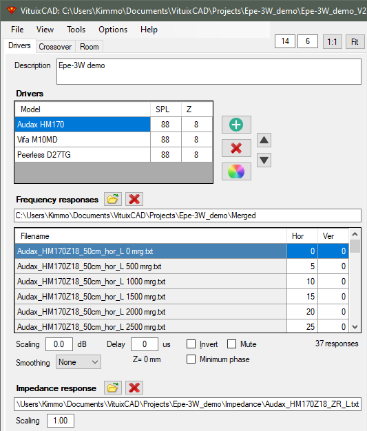
Drivers in the project are listed in Drivers table. Give actual name for initial dummy driver "Driver #1". Add the rest with (+) button and enter actual names. Enter nominal SPL and Z if you're making just simple tests without measured or simulated frequency and impedance responses. That will scale flat default responses without adjusting via Scaling text boxes.
Click color palette button on the right side of Drivers table to adjust color, width and dash style of driver traces in SPL, GD & Phase, Filter and Power dissipation charts. Different settings for six driver models are available. Magnitude and phase responses can have different properties.
Filenames must have valid coding for plane and off-axis angle.
ARTA style angle coding <name-prefix>_deg[+|-]<num>.txt is okay, as well as CLIO style <name-prefix> <num>.txt where angle <num> is multiplied by 100.
Different planes should be separated with a keyword, typically 'hor' or 'ver'.
For example 'M15CH002_hor_deg+110.txt' or simply 'M15CH002 hor 110.txt' equals to M15CH002 to horizontal off-axis angle of 110 degrees with angle multiplier 1.
'M15CH002 hor 11000.txt' equals to horizontal 110 deg with CLIO naming style having angle multiplier 100.
3D balloon data with CLIO, EASE and VACS file naming formats is also supported. Program is able to read horizontal (phi=0) and vertical (phi=90 deg) planes from balloon data. Rotation of phi by +90 deg may be needed if balloon data is captured with Klippel NFS. See Options for more information.
'SPL Horizonal.txt' and 'SPL Vertical.txt' multi-column files exported from Klippel are splitted automatically into multiple frd files when loaded to Frequency response list in Drivers tab. txt extensions will be renamed to nfs before splitting and loading. Number format should be invariant so comma (,) is not accepted decimal separator. Note! Files don't include measured phase by default so they are not valid for designing multi-way speaker or phase equalization (to get minimum-phase response).
Add driver's frequency responses by clicking open button or dropping files into response list. All files of the driver should be selected in one pass with multi-selection (Ctrl or Shift key pressed) i.e. files should locate in the same folder. Delete button X clears response list.
Maximum of 718 frequency responses per driver is supported in practice. Angle step of drivers' off-axis responses could be denser, fewer or equal to angle step of simulation set in Options window. Measured angle step could be constant (0, 10, 20, 30, ..., 180) or variable (0, 5, 10, 15, 20, 30, 40, 50, 60, 80, 100, 120, 150, 180). Off-axis responses of different driver types can have different angle step - constant or variable.
Power response and directivity index are calculated within minimum coverage angle of drivers' frequency responses i.e. 0-180 deg must be measured for all drivers in order to calculate power and directivity to full space.
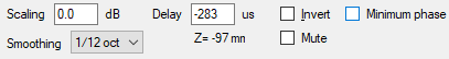
Frequency responses can be scaled (dB), smoothed (none, 1/24, 1/12, 1/6, 1/3, 1/2 oct.), delayed (± µs), polarity inverted, muted and converted to minimum phase with controls below frequency response list. Hor and Ver angle can be modified by entering new value to the field if program fails to parse angle value from the filename or measurements are swapped intentionally.

Reference angle is direction in horizontal plane which is shown as On-axis/Ref axis response in SPL, CTA-2034 and Phase response graphs. Also directivity index calculation can use reference angle instead of Listening window. See CTA-2034-A in Options for more information. Optimizing to single off-axis direction is useful if On-axis response is bad or not representative or measurement data is poor and accurate power response is not available. Default value is 0 deg hor.
Select impedance response file for a driver(s) by clicking folder button or dropping file into text box.
Impedance response can be scaled as well with a multiplier. If multiple drivers are entered to crossover as a single driver (not recommended), scaled impedance response should represent total impedance of driver group. If impedance response was measured from group of drivers in common volume and drivers are entered to crossover as a single drivers (as recommended), scaled impedance response should represent single driver.
VituixCAD supports tab, space or semicolon delimited .txt or .frd or .zma (for impedance). Recommended decimal separator is period (.). Comma (,) is used as decimal separator if data line doesn't contain periods. Comma is used as field/column separator if data line contains both periods and commas. Therefore any thousand separator is not allowed. Following software exports are supported:

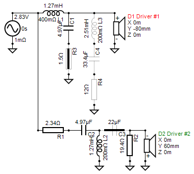
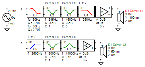
Unlimited amount of components can be added via Crossover component menu. Menu includes generic active blocks (9), active transfer function file, operational amplifier, passive components L C R T, library block (LIB), comment text (T), wire, ground and driver.
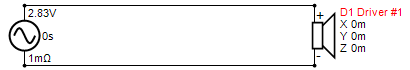
Crossover should contain one Generator. No more - no less. Parameters are source voltage Eg and output impedance Rg. Voltage affects to sound pressure level in SPL, CTA-2034 and Directivity graphs, but not to Power dissipation window having own signal. Level in SPL plots equals to USPL when frequency responses in Drivers tab are scaled to dBSPL/2.83V and Ug=2.83 V.
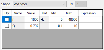
Active Low pass and High pass filters (f). Shape and Order are selected from list boxes:
Active Shelving Low pass and High pass filters (f, gain). Shape is selected from list box:
Active Linkwitz Transform (fo, Qo, fp, Qp)
Active All-pass filters (f). Shape and Order are selected from list boxes:
Active Peak/Notch filters. Type is selected from Shape list box:
Active Slope filter (f, S).
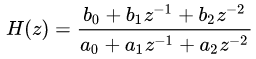
Digital Biquad (b0, b1, b2, a0=1, a1, a2)
Active Buffer / Power amplifier of active multi-way (gain dB, delay µs, polarity inversion)
Operational Amplifier (open-loop gain AOL, gain bandwidth product GBP)
Transfer function file, any supported frequency response file type
Passive R (maximum power Pow W)
Passive C (series resistance ESR Ohms)
Passive L (series resistance DCR Ohms, Wire diameter mm, parallel resistance Rpar Ohms, parallel capacitance Cpar uF).
Rpar is included in calculation if Value < 1 MOhms. Power dissipation of Rpar is ignored.
Cpar is included in calculation if Value > 100 pF.
Passive ideal Transformer (N=Vs/Vp)
Driver (X,Y,Z mm, R,T deg). See 'Driver instances' below
Generator (Eg Vrms, Rg Ohm)
Important! Active filters in blue are NOT minimum-phase. Blocks in the schematic have 'FIR' text for information. Convolver plugin or DSP device with FIR features is needed for real life application. Transfer function of active filters per driver can be exported as impulse response in wav or txt file format. See section Impulse response.
Components are added by clicking menu button, moving to correct location and clicking left button. Esc key, right click or clicking menu button X cancels adding.
Selected component can be replaced by pressing Ctrl key while clicking menu button. Active block can be replaced with another active, and passive component (LCR) with another passive. Values of parameters with the same name and unit are copied to replacement component. Driver, ground, library block and wire cannot be replaced directly without delete->add.
Each driver instance added in the crossover can be provided with location relative to "design origin". Location is entered to Parameters grid. Design origin is typically perpendicular endpoint of listening axis on front baffle surface. X [mm] is horizontal coordinate of center point; negative to left and positive to right (mic/listener view). Y [mm] is vertical coordinate; negative down and positive up (mic/listener view). Z [mm] is horizontal distance coordinate; negative closer to mic and positive further from mic.
Horizontal rotation R [deg] and vertical inclination T [deg] of drivers are also supported. Rotation R [deg] is positive to counter-clockwise from top view, and inclination T [deg] is positive to up.
Measurement data in Drivers tab is linked to driver instance in crossover network with a list box located below crossover schematic. List box is visible when driver is selected in crossover.
Multiple drivers should be entered as a single driver if they are measured in the prototype cabinet as a package; all connected to power amplifier at the same time. Location is entered as a difference between measurement and design origins.
Example 1: Location (X,Y,Z) = (0,0,0) if multiple driver package is measured on design (listening) axis.
Example 2: Location (X,Y,Z) = (0,-400,0) if multiple driver package is measured 400 mm below design (listening) axis.
Library block menu can be filtered shorter with checkboxes in Filter group. See searched keywords from tooltip of each checkbox. Block is inserted to crossover by double-clicking or with Open button. Blocks (vxl files) are also possible to drag & drop with file system from VituixCAD\Library folder to crossover.
See also VCLLabs opamp filter blocks

Library block could have attributes for calculating component values by user parameters and mathematical expressions. Tune block window opens when block is inserted, or Tune block... is selected from context menu. Values are updated to crossover while parameters are adjusted. Attribute values can be solved with Optimizer by checking Opt.

Purge command disconnects links between block and components, and clears expressions from component parameters which enables modification of previously calculated parameters. Purged block disappears when project file is saved.
Wires are added by point & left click, point & left click etc. Space or Enter key or right click accepts/terminates wiring. Esc key rewinds wire node by node until all nodes are removed. Wire is highlighted with lime color when cursor is at valid termination point i.e. terminal of a component, or existing node or endpoint of another wire. New node is created if wire is started or ended to intermediate point of existing wire, or terminal of component is dropped into intermediate point of existing wire in the end of dragging (adding or moving).
Wire can be started from existing wire node or component terminal without clicking wire button in component menu or W shortcut key. Creating new node to intermediate point of existing wire requires wiring command.
Red terminal dot of component indicates missing connection. Program can handle unconnected terminals but calculation speed is reduced.
Shortcut letter keys are available for adding the most common passive components:
C for capacitor, L for inductor, R for resistor,
M for transformer, W for wire, G for ground, T for comment text and D for driver.
Passive components and texts are added as rotated (=vertical) if Shift key is pressed while clicking component menu or shortcut letter key.
Components can be selected for modification by clicking or window selection. Multi-selection with Ctrl or Shift key pressed is available for both clicking and window selection. Selection set is reset by clicking empty area. So called 'Top component' is one of the selected components which parameters are show in Parameters grid below the schematic. Top component is emphasized with bold highlight color, typically blue. Other selected components (except Top component) are emphasized with semi-transparent highlight color, typically light blue. All selected components are targets for moving or modification with context menu or shortcut keys.
Selected components can be moved by dragging with mouse or arrow keys. Wires connected to terminals of moving component are stretching along if component is moved by dragging and Stretch is checked. Components are disconnected from the network without wire stretching if moved with arrow keys or Stretch is unchecked while dragging. Pressing Alt or Shift key while dragging inverts the setting on the fly.
Context menu shows possible (and few impossible) actions for the selected components. See also shortcut keys.

| Tune block... | Opens window for adjusting user parameters of selected block. |
| Pan to center | Point of mouse cursor scrolls to the center point of picture area (as center as possible). |
| Undo | Up to twenty most recent changes and situations before parameter adjustment can be restored. |
| Redo | Reverse Undo commands. |
| Select all | Selects all components in the crossover. |
| Cut | Cuts selected components to the clipboard. |
| Copy | Copies selected components to the clipboard. |
| Copy Biquad coeffs | Opens Copy biquad coefficients -window. See Biquad coefficients below. |
| Paste | Pastes from the clipboard to cursor position. |
| Paste Biquad coeffs | Pastes first coefficients from clipboard text to selected Biquad blocks. Note! Format should be miniDSP compatible i.e. Block type, Biquad number, a0, Parameter name, Value as decomal and End comma should be checked. |
| Delete | Deletes selected components. Deletion of the last generator is verified because network should contain one generator. |
| Open | Disconnects selected components from the network. Active blocks are disconnected by setting gain to 1E-10. Opened components are visualized with transparent color. |
| Short | Selected components are shorted (bypassed with wire). Active blocks are shorted by setting gain to 1. Shorted components are visualized with thick black line over the component's body. |
| Invert | Polarity of selected components is inverted. Applies to Active Buffer and Driver. Visualized with +/- signs in schematic. |
| Mute | Selected drivers are muted. Driver is electrically in the network, but acoustical output is muted. |
| Rotate | Selected (passive) components and comment texts are turned vertical. Single component is possible to rotate with right click while dragging. |
| Hide traces | Chart traces of selected drivers are hidden. |
| Raw response | Shows raw response of driver without crossover. |
| Optimize On | Main parameters* of selected components are selected for optimizing. Optimized parameters are visualized with semi-transparent pale green background in the schematic. *Main parameters of passive components are L, C, R. All parameters of active blocks are main parameters except AOL and GBP of OP amplifier. Main parameters of Drivers are X, Y, Z (location in mm). Other parameters should be selected for optimizing via Opt column of Parameters grid. |
| Optimize Toggle | Optimize status of selected components is inverted. This enables swapping of two component groups without changing selection set. |
| Optimize Off | Optimize status of selected components is reset. |
| Part numbers > | |
| Number blanks | Renumbers components with empty Part # starting from the next free number. Part # text box is green while numbering mode is on. Numbering is done by clicking components in desired order. Numbering mode ends by clicking empty area or right click or Esc. |
| Renumber all 123... | Renumbers all components starting from 1. Numbering is done by clicking components in desired order. |
| Clear selected | Clears Part # of selected components. Helpful before Number blanks command. |
| Clear all | Clears Part # of all components. Helps detection of unnumbered while Renumber all. |
| Driver layout... | Opens table view for modifiying driver locations or creating line array. |
| Copy image | Copy crossover schematic image to clipboard |
| Export image | Export crossover schematic image to file. |
Buttons located below crossover schematic:

| Open | Same as Open command in context menu. Shortcut key is Ctrl+O. |
| Short | Same as Short command in context menu. Shortcut is Ctrl+S. |
| Invert | Same as Invert command in context menu. Shortcut is Ctrl+I. |
| Mute | Same as Mute command in context menu. Shortcut is Ctrl+M. |
| Rotate | Same as Rotate command in context menu. Shortcut is Ctrl+R. |
| Hide | Same as Hide traces command in context menu. Shortcut is Ctrl+H. |
Visualization of component status:

In addition to normal text, comment could contain single link to local file or several URL-addresses separated with space or new line. Comment text with URL(s) could contain normal text before, between or after the link(s). All URLs are opened at once by single double-click. Links are opened with desktop application if link text starts with application's name: for example onenote:https:// and Shift key is pressed while double-click.

Sign of coefficients a1 and a2 is negative and a0 is normalized to 1.
For example 3rd order Butterworth LP 1000 Hz:
Coefficients are compatible with 'Cookbook formulae for audio EQ biquad filter coefficients' by Robert Bristow-Johnson.
Exception: coefficients are normalized to a0=1 with Generic DSP.
For example 3rd order Butterworth LP 1000 Hz:

Selected IIR blocks can be copied or exported as digital biquad filter coefficients b0...a2.
Also parameters of active buffers is possible to copy/export.
Checking 'Block type' adds 'biquad' or 'buffer' text before coefficient/parameter lines.
'Biquad number' adds consecutive number for each biquad.
'Buffers' shows gain, delay in samples, invert and unmute parameters of active buffers.
'a0' shows coefficient a0 no matter is it normalized to 1 or not.
'Parameter name' shows the name of each coefficient (b0=, b1=, b2=, a0=, a1=, a2=) or parameter.
'Value as decimal' or 'Value as 8.24 hex' or both show value of coefficient/parameter.
'End comma' adds a comma to the end of all lines.
Copy button copies whole content to the clipboard. Export button allows saving directly as a text file for loading to another application such as AD SigmaStudio. Selected part of the text can be copied to the clipboard with Ctrl+C or right click Copy.
Minimum eight (8) biquad blocks are created if DSP system is miniDSP and Shift key is pressed while copy/export command.
Note! Select correct DSP system from Options window before copying biquads. FIR, transfer function file, passive and open/shorted blocks are ignored. Stability of biquad filters is not checked.

Checking 'Replace variables' enables creating EQ settings text file from a template (.vxt by default).
Template file contains static text and variables which will be replaced with coefficient/parameter values in the text box.
Values can be either decimal or 8.24 hex depending on target system.
Format of variables is '$(' + name + ')'.
Name is generated from Part # + colon (:) + coefficient/parameter name. For example:
$(U11:b0), $(U11:b1), ..., $(U12.1:a2) is 2nd order IIR block, Part #=U11.
$(A11:gain), $(A11:delay), $(A11:unmute), $(A11:invert) is buffer block, Part #=A11.
Note! Buffer's gain is absolute 10^(dB/20), delay is rounded to samples, muted=0 and inverted=1.
Period (.) + consecutive number 1-4 is needed after Part # if order of LP/HP filter block is higher than 2. For example:
$(U12.1:b0), $(U12.1:b1), ..., $(U12.1:a2) is 1st stage of Part #=U12.
$(U12.2:b0), $(U12.2:b1), ..., $(U12.2:a2) is 2nd stage of Part #=U12.
Generic variables:
$(filename) is project filename without directory and .vxp extension.
$(description) is Description text visible in Drivers tab.
$(variant) is crossover variant 1-8.
Click Replace button to create and save EQ settings file. Default extension is .txt.
Click 1:1 button to zoom schematic picture to nominal 10 pixels/snap unit.
Click Fit button to fit components into picture area (within limits of zooming range).
Picture can be zoomed in/out with Ctrl + mouse wheel. Zooming range is 70%...300% from nominal 10 px/snap unit.


Selecting of component opens corresponding parameters to the list and shows additional list boxes. Component values can be entered directly to the Value field. Value field accepts metric prefix: p,n,u,m,k,M,G,T. Additionally, component value can be increased/decreased by Alt+Up/Down key or arrow buttons on the right or mouse wheel. Parameter can be adjusted with mouse wheel over the selected component. Increment is defined by component Snap value. Available values are 5 %, E12, E24 or E48.
Parameter will be included in frequency response optimizing if Opt field is checked. Otherwise parameter is excluded and existing value locked. See Optimize.
Min and Max fields limit parameter value while manual adjustment and optimizing.
Expression field could contain variable name or full expression for calculating parameter value. Calculated values are readonly with gray background. See Library blocks.
Variants are different development stages of the crossover or versions for different drivers or DSP gear/app.
S# (save) button creates a copy (exact clone) of visible schematic to selected variant memory.
All changes are saved automatically to visible variant. No need to click S# button again.
Enabled R# (recall) button indicates that the variant exists.
Existing variant is loaded to schematic with R# button.
Other variant is possible overwrite with visible schematic by clicking S# button with already enabled R# button.
Program asks confirmation 'Overwrite existing crossover variant #?'.
Variant can be deleted by pressing Ctrl-key while clicking R# button. Program asks confirmation 'Delete crossover variant #?'.
Crossover variants are saved to project file (.vxp) for the next session.
#1 is compatible with the oldest project file versions of VituixCAD 2.0.
Warning! Undo buffer is cleared when variant is changed with S/R button.
Driver layout window allows changing of part #, location (XYZ), rotation (R) and tilt (T) of drivers with table control, or adding new drivers as linear or curved array.
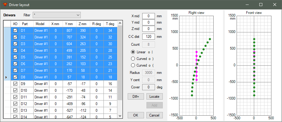
Drivers table contains existing driver instances in the crossover. List can be filtered with Filter combo box. Rows can be sorted by Part # or Y mm by clicking column header. XO cell is checked if driver exists in the crossover.
Green dots in graphs show existing locations in Drivers table (initially existing locations in the crossover). Magenta dotted line/curve shows locations calculated with line array parameters (in the middle) but not yet accepted to Drivers table.
Parameters of line array calculator:
| X mid | Horizontal location of array's middle point, relative to listening axis. |
| Y mid | Vertical location of array's middle point, relative to listening axis. |
| Z mid | Distance offset for array's middle point, relative to origin i.e. endpoint of design/listening axis on baffle surface. |
| C-C dist | Distance between drivers from center to center. Along circumference with curved arrays. |
| Count | Numbers of drivers in array. Enabled while adding new drivers. |
Array types
| Linear | | Straight vertical line. |
| Curved o ) | Curved array where focal point is in front of speaker. |
| Curved o ( | Curved array where focal point is on the back side of the speaker. For example CBT. |
Parameters for curved arrays
| Radius | Radius of curved array. |
| Y cent | Vertical location of curve's center point, relative to listening axis. |
| Cover | Calculated coverage angle of 'slice'. |
Parameters Part #, X, Y, Z, R and T can be modified manually to the grid. Accept changes to crossover and close window with OK button. Cancel button closes the window without saving changes to the crossover.
Drivers can be renumbered by entering first Part # to the top cell, selecting cells to be renumbered (including the first cell) and clicking D#+ button.
Select full rows with top left corner or row headers in order to calculate new locations and tilts with line array parameters. Select array type, adjust parameters until magenta dotted curve is okay and apply changes to Drivers table with Locate button.
Select driver with Filter combo box in order to add new drivers to the table. Full rows should not be selected. Select array type, adjust parameters until magenta dotted curve is okay and add drivers to the table with Add button. Locations can be modified with calculator by selecting new drivers as full rows. Accept changes and new drivers to the crossover with OK button. New drivers will be added as max. 8x8 matrix beginning at constant location 43,9.
New library block is created by selecting components from crossover and then File->Create library block. Block attribute editor opens. Program lists all parameters of selected components into Component parameters grid. User has few choices:
a) If components could have different values depending on filter variation e.g. Bessel or Butterworth, enter variable name into Expression field of component, and add variable with mathematical expression to Block attributes list.
b) If the block does not have variations and component values can be calculated directly from user parameters, formulas can be located in Expression field of component parameters.
c) Mix of previous. Intermediate results could be worth to calculate with expressions in block attributes to make component expressions shorter (less repeating). Calculation order of block attributes is from top to bottom.
Examples: formulas in block attributes (left), formulas in component parameters (right).
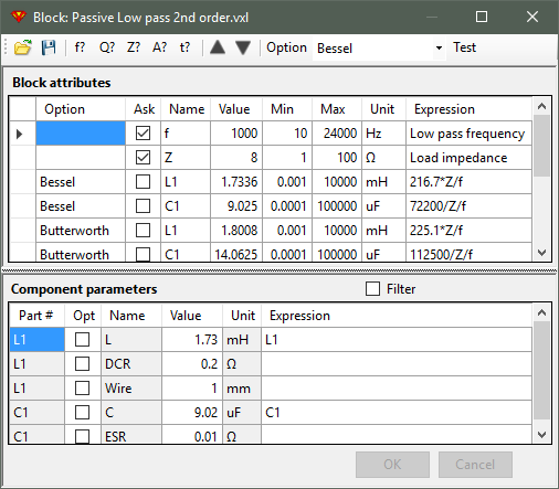

Check Ask field for user questions. Rows can be added manually or initiated with shortcut buttons: f? (frequency), Q? (Q factor), Z? (impedance), A? (gain), t? (time). Option field is left empty (or *) if the row applies to all variations, or block doesn't have variations. Value field holds initial/default value. Calculated values are also limited within Min...Max. Unit and Expression fields are visible for information in Tune block window.
Variable name should begin with letter, lower or upper case. If the name contains numbers, they must be in the end.
Supported mathematical and logical operators: ^, +, -, /, *, %, >, <, ==, &&, !=, ||, !, >=,<=
Functions: cos, sin, tan, acos, asin, atan, cosh, sinh, tanh, cotan, acotan, exp, ln, log, sqrt, round, ceil, floor, abs
Constants: euler, pi, infinity, true, false
Parentheses: (, )
Note! Decimal separator in Expression must be period (.)
Row order can be changed with Up/Down arrow buttons. Initial/default option is selected with Option combo box. Expressions are evaluated to Value cells with Test button, or by changing Option.
Context menu contains: Cut, Copy, Paste, Delete (rows), Duplicate (rows), Append (rows) and Replace.
Press F2 to modify cell value.
Continue with OK button when block attributes and component parameters are okay. Filename is selected in the following Save as dialog. Image visible in library block menu is png-file created automatically when block is saved.
Attributes of existing library blocks can be modified with File->Edit library block parameters command. Open block with small open button in tool strip on the left. Save button overrides existing block without verification.
Response with room reflections visible in CTA-2034 graph can include left side wall, front wall, floor and ceiling, selected with checkboxes in Room tab. Distance from speaker's origin (0,0,0 mm) to reflecting surface and rotation away from left side wall (toe-in) are adjusted with text boxes. Left wall X and Floor Y are negative values. Adjustable absorption in dB is available for both walls, ceiling and floor. Distance equals to Listening distance setting in Options window: distance from speaker's origin to virtual mic/ear.
Locations and reflection 'rays' and exit angles are visualized in Room tab from top and left views.
Room response with reflections is scaled -10 dB to fit in CTA-2034 chart. Predicted in-room response /CTA-2034-A is hidden while response with reflections is visible.

Note! Full 0-180 deg measurement data with Mirror missing is needed to simulate front wall reflection.

Simulated horizontal and vertical planes can be rotated -90...+90 deg around speaker's origin (X,Y=0,0) with Planes [deg] parameter. Both simulation orbits of virtual microphone are rotated around Z-axis by given angle phi. Positive value to counterclockwise.
All driver instances in crossover can be moved temporarily with X,Y [mm] parameters. This enables for example simulation of different listening elevations and very small off-axis angles (within reference angle steps) without permanent relocation of driver instances in crossover. Positive X to right and positive Y to up.
All driver instances in crossover can be rotated or tilted around speaker's origin (X,Y,Z=0,0,0) temporarily with R [deg] and T [deg] parameters.
Driver instances in crossover are moved by X and Y, rotated by R and tilted by T permanently with Relocate button (which also resets X, Y, R and T).
Check 'Rotate 180 deg' to rotate speaker 180 degrees in horizontal plane.

By default, SPL graph shows total SPL, Listening window, target, SPL per individual driver and normal phase. All traces are responses to reference angle, see Frequency responses. Color coding for traces:
SPL Target can be adjusted by dragging the line ends with mouse while Shift or Control key is pressed. This is target for optimizing reference axis response. See Optimize.

Traces... command in context menu of chart opens properties window
allowing user to change visibility, description, color(s), line width and dash style of each trace.
Selected overlays are removed with 'Delete sel' button.
All overlays are removed with 'Delete all' button.
Data points of all or selected traces are exported and copied to clipboard with 'Export data' button.
Hold Shift key to reverse column order of Y values.
Number format of txt file is invariant: decimal symbol is period (.) and no thousand separator.
Number format and list separator of csv file is defined in Windows Control panel.
Multi-selection with row headers or top left corner.
Line color and fill color with Waterfall and Surface charts is selected from list of 'named colors' or with standard Colour dialog.
Default color selection window can be changed by pressing Ctrl-key while clicking color cell in Traces window.
Dash style is selected with combo box.
Available styles are Solid (default), Dash, DashDot, DashDotDot and Dot.
Color BW (black & white) button changes selected/all traces to text color and area fill to background color of chart.
WB (white background) button changes area fill to background color of chart.
Line width '1 px' button changes line width of selected/all rows to 1 px.
'2 px' button changes line width to 2 px.
Style Solid button changes dash style of selected/all rows to Solid.
Dash button changes dash style to Dashed.
'Phase Dash' button changes dash style of phase responses to Dashed.
Save as overlay in context menu of chart saves selected (bold) trace, or all visible traces as overlays if none is selected. Overlay traces are not possible to overlay again.

Traces in all graphs are saved as overlays with Ovl (+) button above the graph 6-pack. Content of text box on the right is added as name suffix for each overlay trace. Overlays in all graphs are cleared with (-) button.
Open overlay... command in context menu opens standard open file dialog for selection.
Response files (txt, frd, lms, zma) can be loaded as overlay traces.
Select 'Left Y axis' or 'Right Y axis' or 'Both' if chart has two axles.
Dropping files into chart area with Drag & Drop is also supported.
Traces are scaled with Left Y axis if the files are dropped closer to Y axis on the left.
Traces are scaled with Right Y axis if the files are dropped closer to Y2 axis on the right.
Selected overlay can be scaled with Shift + mouse wheel or Ctrl + Shift + mouse wheel.
All visible overlays are scaled if none is selected.
Total number of traces including overlays is limited to 37 per chart.
Copy image command in context menu of chart copies image to the clipboard as bitmap. Legend area with trace names is included. Image size excluding legends is specified in Image export -group in Options window.
Copy six-pack command copies all six charts to the clipboard as a bitmap. Legend areas are not included. Image size of each chart is specified in Image export -group in Options window.
Export image command in context menu of chart exports image to a file. Supported file formats: PNG, BMP, EMF, EXIF, ICON, JPEG, GIF, TIF, WMF, SVG. Recommended formats are PNG and SVG. Legend area with trace names is included. Image size excluding legends is specified in Image export -group in Options window.
Export all images command gives 'Export image' command for all six charts. Legend areas are included.
Export six-pack command exports all six charts to a single file. Legend areas are not included. Image size of each chart is specified in Image export -group in Options window.
Y-scale maximum of SPL, CTA-2034 and unnormalized Directivity charts is adjusted automatically by default.
Manual setting with text box is possible by checking SPL max on the left side of SPL chart.
Manual value is saved to project file.

Span (dB range) of SPL, CTA-2034 and Directivity charts can be adjusted with Expand SPL scale and Compress SPL scale buttons. Available spans are 20, 25, 30, 35, 40, 45, 50, 60, 70, 80 and 90 dB. Initial value is defined in Options window.
In addition, Y-axis maximum can be adjusted with mouse wheel, and span (dB only) with Ctrl + mouse wheel when mouse cursor is closer to Y-axis on the left. Exception: Directivity chart follows max and span settings of SPL chart.
Y2-axis maximum can be adjusted with mouse wheel, and span (dB only) with Ctrl + mouse wheel when mouse cursor is closer to Y2-axis on the right. Exceptions: Directivity index has common span with SPL, and maximum is span - major grid interval. Phase angle has constant Y2-scale +180...-180 deg.
Every graph can be zoomed to full size and back to dashboard by double clicking in middle of the chart area.

This graph shows On-axis/Ref axis total SPL (WindowFrame), Listening Window (YellowGreen), Predicted In-room /CTA-2034-A or response with 1st order room reflections (DarkOrange), Sound Power (Blue) and Sound Power DI (Red).
Show Slope target zones toggles visibility of recommended slope target range for ON-LW, PIR, SP and SPDI @100-16000 Hz.
Show Basic command shows On-axis/Ref axis, Listening Window, Predicted In-room, Early Reflections, Sound Power, Sound Power DI and Early Reflections DI.
Hides Wall, Floor and Ceiling Bounces, Vertical Reflections, Vertical Reflections DI, Horizontal Reflections and Horizontal Reflections DI.
Show Early Reflections command shows Front Wall Bounce, Side Wall Bounce, Rear Wall Bounce, Floor Bounce, Ceiling Bounce and Early Reflections.
Hides On-axis/Ref axis, Listening Window, Predicted In-room, Sound Power and Sound Power DI.
Shows also temporary 'Early Reflections' text in chart title.
Show Reflection totals command shows Vertical Reflections, Vertical Reflections DI, Horizontal Reflections and Horizontal Reflections DI.
Show Predicted In-room toggles visibility of Predicted In-room response.
Show Data labels toggles visibility of smoothness (SM) and slope in dB/oct of ON, LW, ER, PIR, SP, SPDI and ERDI @100-16000 Hz.
Normalized shows flat frequency response to reference angle.
Download Standard Method of Measurement for In-Home Loudspeakers (ANSI/CTA-2034-A R-2020) for more information. See tooltips or Traces... to identify curves. See Chart overlays.
There is also adjustable target curve (magenta), normally set for sound power (blue). Target can be adjusted by dragging the line ends with mouse while Shift or Control key is pressed. This is target for power response optimizing. See Optimize.


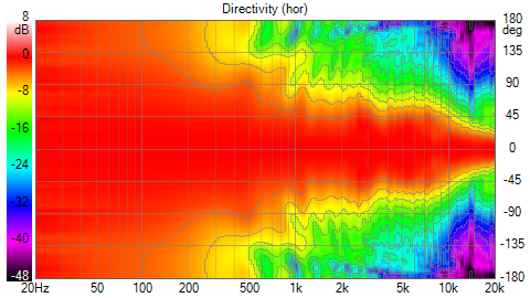
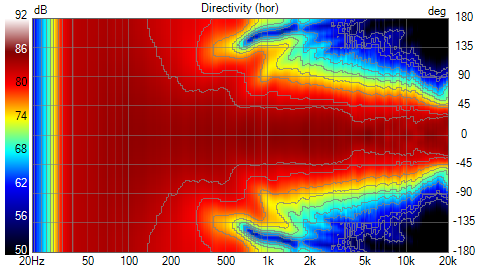

This graph shows directivity simulation as line chart, waterfall, surface chart, polar map (aka heat map) or polar chart.
Density of simulated off-axis directions is selected with Angle step list box in Options window.
Response to reference angle is emphasized with thick line (except Polar map).
Line chart: Trace below mouse cursor is highlighted.
Highlighting is possible to lock by clicking the curve.
Unlock by clicking chart area.
Waterfall: Highlighted off-axis trace is selected with mouse wheel.
Frequency is adjusted with mouse move left/right.
Depth is adjusted with left mouse button + mouse move up/down (or Ctrl + mouse wheel).
Surface: Image rotation and inclination is adjusted with left mouse button + mouse move.
Limits for rotation and inclination are 10...170 deg.
Image size/distance is adjusted with mouse wheel.
Image is panned with Ctrl + mouse move.
Depth is adjusted with Ctrl + mouse wheel.
Polar chart: Frequency is adjusted with horizontal scrollbar below chart area.
Directivity chart options context menu (right click on the graph):

Checking User's off-axis angles will show directions listed in Options window (except Polar chart).
Checking Show ±90 deg hides off-axis angles outside half space.
Checking Show ±45 deg hides off-axis angles outside eighth space.
Checking Negative angles in front will invert angle-axis of the plot.
Checking Normalized will show flat response to reference angle.
Checking Contour lines 🠞 Show will show edges of level ranges with Polar map.
Level step can be selected from submenu: 1, 2, 3 or 6 dB.
Number of contour lines can be selected from submenu: 1, 2, 3, 6 or 10 lines.
Klippel palette starts with dark red, ends with dark blue, contains much less green and no magenta compared to palette using full linear color circle.
Adjust depth allows angle axis scaling of Waterfall and Surface chart by entering value.
Temporary adjustment of colors, line width and description of traces is available with Traces... window.
Save as overlay is available for Polar chart only.
Chart title shows visualized plane. 'hor' and 'ver' texts indicate nonrotated planes. If simulated planes are rotated around Z-axis with Microphone offset Planes [deg] parameter in Drivers tab, chart title shows azimuth angle phi of visualized plane. Phi range is -45...hor...+45 deg when Horizontal plane is selected from context menu of Directivity chart. Phi range is +45...ver...+135 deg when Vertical plane is selected from context menu.

This graph shows Normal group delay (WindowFrame), Normal phase (gray) and phase response of individual drivers to reference angle. Optional Excess group delay (SteelBlue) is enabled by checking Show Excess group delay in context menu. Group delay can be hidden by unchecking Show Normal group delay. Total phase can be hidden by unchecking Show Normal phase. Unit of group delay traces is changed from milliseconds (ms) to cycles (cyc) when Normalized is checked. Selected (bold) phase serie is normalized to 0 deg line when Normalized is checked.
See tooltips or Traces... to identify curves. See Chart overlays.

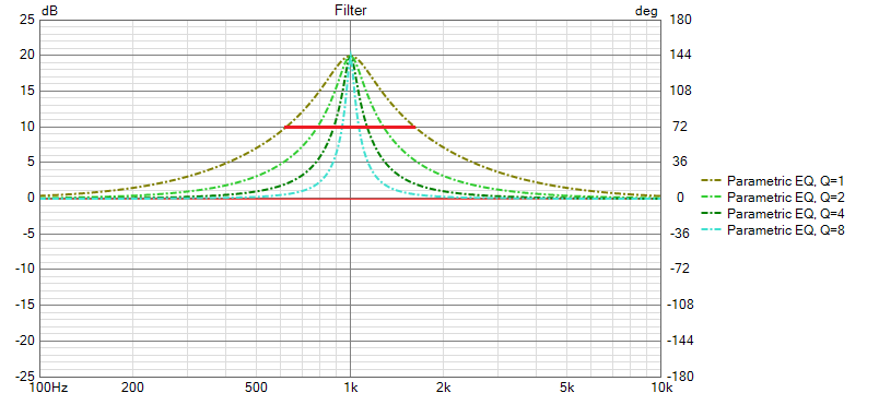
This graph shows magnitude of filter transfer function of individual drivers. In addition, graph shows magnitude and phase response of selected active block (Highlight color).
See tooltips or Traces... to identify curves. See Chart overlays.
There is also optional target magnitude curve (Magenta). This is target for optimizing filter transfer function of driver. See Optimize.
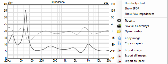
This graph shows generator's load impedance magnitude (WindowFrame) and phase (Gray). In addition, graph shows total and individual load impedance of active buffers in active multi-way system, 'Equivalent Peak Dissipation Resistance' EPDR (Dark Violet) calculated from generator's load impedance and raw impedance responses of driver models in Drivers tab. Active buffers can also be used in passive system for measuring impedance of separate ways without opening components. Note! Impedance chart can be replaced with second directivity chart e.g. to show both planes at the same time. Visible chart is selected with context menu.
See tooltips or Traces... to identify curves. See Chart overlays.
Optimizer adjusts selected filter parameters/component values to shape total reference axis response or listening window and power response or predicted in-room, or driver's on-axis response or transfer function magnitude at driver terminals to target specified by user. Optimizer window can be activated with context menu of SPL or CTA-2034 chart.

Frequency range included in optimization is limited with two frequency values. Target response outside specified limits is not visible in the graph.
Target curve could be either frequency response File (txt/frd) or ideal Texbook response with adjustable tilt, high-pass and low-pass slopes.
Target SPL and Tilt can be adjusted manually using the text fields, or read automatically for driver's on-axis target from total SPL target by clicking binocular button. Ends of target lines in SPL and CTA-2034 charts can be set with mouse while left button and Shift or Control key is pressed.
Value in drivers text box scales target SPL by number of drivers with the same polarity and crossover. Enter number to text box or search from crossover with drivers button. Polarity of target response is changed with Invert checkbox.
Filter design is selected from the first dropdown menu (High pass or Low pass).
VituixCAD supports 1st...8th order Butterworth, Bessel, Chebychev 0.5 dB and Linkwitz-Riley, 2nd order with variable Q factor, Duelund and Trifonov Transient.
Bessel slopes are level-normalized i.e. level at given corner frequency is -3.01 dB with all orders, regardless of DSP system selection in Options.
See Appendix 2. DSP dependencies for more information.
10th...16th order Linkwitz-Riley slopes are available as linear-phase only (Lin.pha checked).
Duelund BP (filler middle in 3-way) is set using HP pass section.
Second dropdown menu (N) controls order of the slope.
Corner frequency of the slope is adjusted with the last text field (f).
Linear-phase slope is created by checking Lin.pha, typically for FIR applications.
Note! Order, Q factor, Lin.phase and Invert controls are hidden with Trifonov filters because settings are fixed.
Target curve can also be loaded from frequency response file (txt/frd) with Open button or drag&drop. Target response can be scaled (dB), delayed (µs), polarity inverted, smoothed 1/2...1/24 octs and converted to minimum phase. Frequency range limits effect also to response file. Textbook response can be re-activated by clearing response file with X button.
Target response divided by response to reference angle or listening window can be exported with TF button.
Range equalized with target is set with Frequency range low and high limit.
Check 'Free LF' to export TF with constant gain below frequency range low limit. Uncheck to extrapolate gain below low limit.
Check 'Free HF' to export TF with constant gain above frequency range high limit. Uncheck to extrapolate gain above high limit.
Response file is loaded automatically into Transfer function file G(f) block currently selected in crossover.
This feature can be helpful while designing FIR filters with exported impulse response files because
crossover can include single G(f) block and active buffer for the speaker or each driver/way,
and response is shaped automatically to target; ideal textbook curve with tilt and HP/LP or a file.

Reference axis response of selected driver can be adjusted automatically to the target in SPL graph by selecting 'Ref axis response of Driver'. Select driver from the list box on the right and then 'Ref axis response of Driver'. Create target curve, specify frequency range and select filter parameters/component values to be optimized from Parameters grid in Crossover tab. Driver's target magnitude is visible in SPL graph and target phase in GD & Phase graph. Start solver with Optimize button.
Filter response (magnitude only) of selected driver can be adjusted automatically to the target in Filter graph by selecting 'Filter gain of Driver'. Create target curve, specify frequency range and select filter parameters/component values to be optimized. Target response is visible in Filter graph. Start solver with Optimize button.
Preference rating can be maximized automatically by selecting 'Preference rating'. Calculation is done with the latest settings in Preference rating window.
Total SPL to reference angle or listening window can be adjusted automatically to the target
in SPL graph by selecting 'Ref axis response of Speaker' or 'Listening window'.
Select 'Listening window' if you like to optimize RMS of multiple responses instead of single response to reference angle.
In addition, Sound power response or Predicted in-room can be adjusted automatically to the target
in CTA-2034 graph by selecting 'Power response' or 'In-room response'.
Check 'modify target' to show and edit target in CTA-2034 graph with controls in Optimizer window.
Weighting between SPL and CTA-2034 responses is controlled with percent values.
Higher value produces smaller difference between the target and simulated response.
For example Ref axis/Listening window=60%, Power/In-room=40% allows more error in Power/In-room than Ref axis/Listening window.
That could be better if intended listening distance is very short or room is very damped i.e. decay time is short.
Response is optimized to both shape and level of target curve by checking 'Seek level'.
If unchecked, optimizer does not care about level - just shape within frequency range limits.
Create target curve, select filter parameters/component values to be optimized from Parameters grid in Crossover tab.
Include components with Optimize On/Toggle/Off commands in context menu of schematic.
Start solver with Optimize button.
Optimizer calculates squared error within frequency limits of each target curve.
Check 'Minimum impedance' or 'EPDR' and enter preferred minimum value to text box if you like to control impedance response.
Squared error is increased with penalty function if minimum impedance/EPDR drops below the setting.
Minimum is detected from total impedance while optimizing total SPL and CTA-2034 response.
Check 'Maximum gain' and enter preferred maximum value to text box if you like to limit filter gain.
Squared error is increased with penalty function if maximum gain exceeds the setting.
Maximum is detected from filter of all drivers.
Check 'Ref axis linearity' and enter preferred maximum deviation to text box
to limit difference between maximum and minimun SPL within optimized frequency range:
range of target in SPL chart when Ref axis or Listening window is optimized, 100-16000 Hz when Preference rating is optimized.
Squared error is increased with penalty function if deviation exceeds the setting.
Passive crossover components can be rounded to the closest value in standard E-series by selecting E12, E24 or E48. Note! Values are rounded after optimization which will increase squared error in the end.
Optimization could end up to bad result if initial parameter values are too far from good solution and method finds wrong local minimum. Adjust parameters manually closer to acceptable solution and restart solver with Optimize button. Result can be rejected with Undo button. Undo is able to restore up to twenty most recent changes.
Optimizer stops when error is zero (rarely) or Stop button is pressed or maximum evaluations is reached. Initial maximum is 300 evaluations. Simple problems with only few parameters to optimize could be solved with less than 100 evaluations.
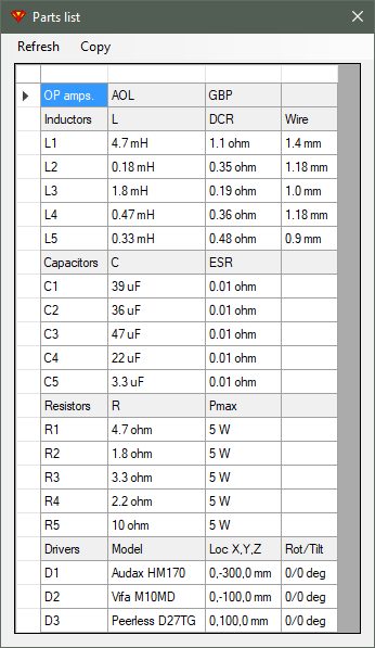
Parts list shows passive components, drivers and parameter values in a grid. List can be copied to your favorite spreadsheet or text editor with Copy command or Ctrl+A, Ctrl+C. Refresh updates the list in case components or values have changed after window was opened.
Ref axis response or input transfer function of driver or output of buffer or total Ref axis SPL or Listening window can be exported to impulse response in time domain. Typical application is to produce impulse response as wav-file for speaker controller with DSP FIR support or convolution plugin.
Frequency response is extrapolated to cover band from 0 Hz to Sample rate / 2 (Nyquist frequency) before inverse Fast Fourier Transform. After inverse FFT, impulse response is multiplied by window function to reduce artifact errors due to spectral leakage.

Sample rate: 44100, 48000, 51200, 88200, 93750, 96000, 176400, 192000, 352800, 384000, 705600 or 768000 Hz.
FFT length: 8192, 16384, 32768, 65536, 131072, 262144 bins.
Frequency resolution of FFT is Sample rate / FFT length.
For example 48000 Hz / 65536 = 0.732 Hz.
Taps: 128...131072 samples.
Maximum taps is limited up to FFT length / 2.
IR window function: Rectangular, Bartlett, Hanning, Hamming, Blackman, Blackman-Harris, Nuttall, Blackman-Nuttall, Cosine 0.50/0.75/1.0 or Tukey 0.25/0.50/0.75.
Check shape and location via graph with adequate time span.
See wikipedia: Window function.
Note: Advanced window functions are designed for spectrum analyzing with high S/N where silent side lobes are required.
IR export works fine with Cosine 0.50, Tukey 0.25 or 0.50.
Pre-delay text box and horizontal scrollbar below shift timing of source frequency response before inverse FFT by increasing phase angle (by delay * frequency * 2pi rad).
Tooltip of the scrollbar shows delay in tap number (1-taps) and percent (%) of taps.
Pre-delay is usually quite close to 0 ms if XO filter contains IIR equalization, but not reduction of excess group delay at low frequencies.
Reducing excess group delay at low frequencies requires impulse with "pre-ringing"
so Pre-delay is usually set close to number of taps to make correction as low frequency as possible.
Pre-delay could be quite centered with hybrid equalization including both excess delay reduction and IIR equalization.
Visible signal is selected with Signal to show list box. In addition to exportable signals, listening window average SPL and total SPL to reference angle can be visialized as minimum phase version to evaluate difference to "ideal" timing. See items 'LisWin SPL MP' and 'Total SPL MP' in 'Signal to show' list box.
Visible curves in Time domain chart are selected with Impulse, dBFS,
Step, RMS, Win and ETC checkboxes.
RMS trace shows quadratic mean of step response after pre-delay.
Points up to pre-delay show step response.
Significantly reduced level compared to minimum-phase equivalent (MP) indicates thin and weak transients.
ETC curve can be smoothed by 0-32 samples with ETC smooth text box.
Checking IR max prevents automatic scaling of vertical (Pa/V) axis.
Maximum Y can be adjusted with the text box.
Curves are updated automatically with selected IFFT parameters when crossover is changed. Time scale can be expanded and compressed with arrow buttons.
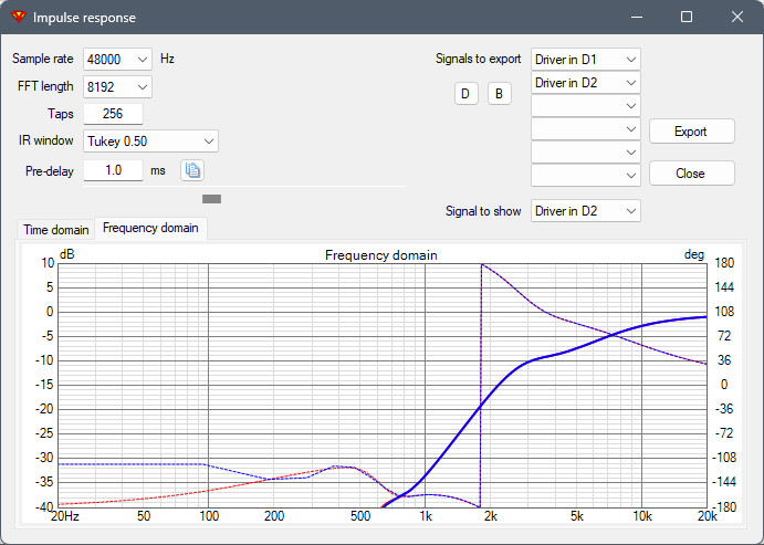
Impulse response with finite length or other modifications usually cannot produce a frequency response that is exactly equal to the source response. Selected window function, location of window function and location of impulse on the time axis also affect the accuracy of the result. Frequency response view (Frequency domain tab) allows you to compare magnitude and phase responses of the selected source response to frequency response generated from impulse response to be exported, so that you can choose parameters that get as close to the target as possible.
Frequency band to be equalized affects the requirements and parameters. For example, high frequencies require less taps than low frequencies. DSP gears have limits in total taps, or some maximum latency cannot be exceed so designer is usually forced to distribute available taps for different channels. For these reasons, impulse responses of different ways may need to be exported with different parameters: number of taps, pre-delay and window function. Different pre-delays need compensation with DSP's delay buffer.
Up to six (6) signals can be exported at once. Signals can be selected manually with Signals to export combo boxes. Driver inputs (max 6) can be selected with D button, and buffer outputs (max 6) with B button. Click Export button to continue. Save as... dialog box proposes project filename + " IR" as a 'root filename'. Select output directory and modify root filename if necessary. Final filename for individual IR-files will be root filename + " Buffer out A1", root filename + " Driver in D1" + extension, etc.
File format is selected in Save as... dialog. File formats:
Electrical signals (Buffer outputs and Driver inputs) exported at once have common scaling factor to maintain gain differences.
Acoustical signals (Driver SPL and Total SPL) exported at once have common scaling factor to maintain sensitivity differences.
Level normalization with WAV files:
Value scaling in text file is equal to source frequency response i.e. not normalized.
Text file has single column from 0.0 s with step of 1/Sample rate [s]:
8.49378929663085E-25
1.64194430575251E-15
-3.17746589425256E-15 ...
Graph shows output spectrum of generator and buffers/power amplifiers in active multi-way,
and power dissipation or current (mA) or voltage of drivers and passive LCR components in crossover network.
Quantity is selected from View group.
Peak voltage (Vp) is shown instead of VRMS by ckecking peak.
Visible curves are selected with checkboxes in Components group.
Curve's tooltip shows part number and name or two main parameters of passive components, including resistance.
In addition, tooltip shows Ptot in watts i.e. total power dissipation of driver, resistor, coil and capacitor.
Calculated as power average within simulated frequency range: sum of power values divided by number of simulated frequency points.
Power should be selected in View group to show Ptot.

Adjustable parameters for output signal from power amplifier or generator:

Purpose of Preference rating (in VituixCAD) is to provide simple target setting and error calculation for the Optimizer.
Rating is calculated with customizable equation using variables described in patent application
US 2005/0195982 A1
by Sean Olive.
Olive's patent application contains many simplifications and negligences measuring just sound balance and coloration with constant signal level.
For example non-linear distortion, dynamics, stability of sound balance, timing, level of directivity, slope of frequency responses and sound power,
diffraction, location of radiators, half space and corner concepts are ignored.
So preference rating alone is not valid design or product ranking benchmark.
Patent application contains also few mathematical illogicalities and conflicts:
Equation including SM_ON, SM_LW, SM_ER, SM_PIR, SM_SP, AAD_ON, NBD_ON, NBD_PIR, LFX and LFQ
with adjustable weight 0-5 for each is available.
Initial weighting factors of variables are visible in the image above.
Equation provides mathematical approach with less illogicalities and conflicts to be valid for optimizing
so rating is not compatible with calculations presented in Olive's patent:
Click 'Full space' button to initialize slope targets for small...middle-sized conventional (boxed) designs.
Click 'Half space' button to initialize slope targets for in-wall and flat on-wall designs.
Click 'Constant DI' button to initialize slope targets for practical constant directivity designs.
Full space and Half space values are compatible with 'Listening window DI' and 'CTA-2034-A power weights' settings in Options.
Traditional DI calculation with single reference angle produces different directivity slopes.
Variables/Columns:
AAD - Absolute Average Deviation (dB) relative to mean level between 200-400 Hz
NBD - Average Narrow Band Deviation (dB) in each 1/2 octave band from 100 Hz - 12 kHz
SM - Smoothness in amplitude response based on a linear regression line through 100 Hz - 16 kHz
slope - Slope of best fit linear regression line through 100 Hz - 16 kHz. Tooltip shows slope in dB/oct and dB/dec.
SL - Absolute difference between target slope and measured slope
LFX - Low frequency extension (Hz) based on -6 dB frequency point transformed to log10
LFQ - Absolute average deviation (dB) in bass response from LFX to 300 Hz
Suffixes of variables in the equation:
_ON - On-axis response
_LW - Listening window
_ER - Early reflections
_SP - Sound power
_PIR - Predicted in-room response
PIR is obtained by a weighted average consisting of:
12 % listening window (LW),
44 % early reflections (ER) and
44 % sound power (SP)

To allow VituixCAD to parse measurement angles and axis from frequency response files, you have to define file naming format/syntax.
Generic 2D is configurable option allowing user to specity how plane and angle value are coded in frequency response filename. Plane keywords define how to distinguish between horizontal and vertical axis. Horizontal axis is selected if keyword of vertical plane is not found in the filename. Search from beginning/end defines whether VituixCAD should start parsing angle value from the beginning of the filename (hor +150 drivername.txt) or the end (drivername hor +150.txt). Angle multiplied by defines how angle value is formatted. For example if 1500 represents 15 degrees off-axis, use Angle multiplied by 100. This option is compatible with ARTA, CLIO in 2D mode.
CLIO 3D filters and decodes either horizontal or vertical plane and angle value from filenames coded by CLIO QC with Auto Save 3-D measurement. The syntax follows: NAME <PHI*100> <THETA*100>.txt/frd. NAME is root filename, PHI is the polar angle (orbit) and THETA is the azimuth (off-axis) angle. These quantities are separated by spaces. Other than PHI=0, ±90, ±180, ±270 are skipped because response file handling and directivity graphs support horizontal and vertical planes only.
EASE 3D filters and decodes either horizontal or vertical plane and angle value from filenames coded by EASE SpeakerLab. The syntax follows: NAME IR[mmm][ppp]. NAME is optional root filename, [mmm] is meridian/orbit and [ppp] is parallel/off-axis angle while the North Pole represents on-axis direction. Other than [mmm]=000, 090, 180, 270 are skipped.
VACS 3D filters and decodes either horizontal or vertical plane and angle value from filenames compatible with Visualizing Acoustics Software (VACS). The syntax follows: NAME Phi[mmm]Theta[ppp].txt/frd. NAME is optional root filename, [mmm] is meridian/orbit and [ppp] is parallel/off-axis angle while the North Pole represents on-axis direction. Other than [mmm]=0, ±90, ±180, ±270 are skipped.
MF 3D filters and decodes either horizontal or vertical plane and angle value from filenames compatible with Four Audio Monkey Forest. The syntax follows: NAME V[mmm]H[ppp].txt/frd. NAME is optional root filename, [mmm] is meridian/orbit and [ppp] is parallel/off-axis angle while the North Pole represents on-axis direction. Other than [mmm]=0, ±90, ±180, ±270 are skipped.
MF 2D is variation of MF 3D. The syntax follows: NAME V000H[ppp].txt/frd for horizontal plane, and V[ppp]H000.txt/frd for vertical plane. NAME is optional root filename and [ppp] is off-axis angle. Other than V000 or H000 are skipped.
Check Swap planes to rotate Phi by +90 deg if balloon data was captured and exported from measurement system so that Phi=0/180 deg stands for vertical plane. Check by default with Klippel NFS.
Test tool is provided for testing the syntax.
Mirror missing defines if VituixCAD should mirror missing measurement data:
Frequency responses are interpolated between off-axis angles and planes loaded to drivers when Interpolate is checked. Program selects the closest off-axis angle loaded to driver when Interpolate is unchecked. This could cause some errors and discontinuities, but enables simple tests and projects with few responses only in Directivity chart.
If crossover of project is active dsp, select exact or compatible device or application from DSP system combo box. Available options are:
Selection has significant effect to frequency response of Active Peak/Notch, Bessel LP/HP and Shelving LP/HP filters, and to highest frequencies due to possible limit in sample rate. Setting is saved in project file (vxp).
Listening distance is virtual distance from loudspeaker to listener or microphone, needed to calculate phase differences and amplitude relations between drivers in different locations. Enter typical listening distance in mm. Default value is 2000 mm.
When Normalize SPL is checked, SPL traces are normalized to level of frequency responses loaded for drivers with generator voltage of 2.83 V. Default value is checked. Keep checked to avoid tuning of SPL and Power targets if listening distance is changed.
Values in Listening window text boxes specify angle range in horizontal and vertical planes included in calculation of 'Listening window average'. See SPL chart and Optimizer.
Off-axis angles listed in User hor and ver text boxes can be shown in CTA-2034 chart. Valid list separators are space, comma or semicolon. Angles should be divisible by Angle step > 0.
Font for crossover schematic and visibility of tooltips are selectable. Check 'Dark mode' to set black background to charts, crossover schematic and room images. Note! Toggling of Dark mode sets default colors to all charts. Check 'Show imperial as tooltip' to show length/diameter/radius, area and volume in imperial unit as a tooltip.
Intensity on spherical surface is normally selected for common sized single or multiway speakers. Intensity on spherical surface around speaker is calculated from radial measurements in horizontal and vertical planes.
.png)
.png)
Intensity on cylinder surface is practical selection for long line sources, or if either horizontal or vertical directivity is temporarily interesting - not accurate power response & DI result. Intensity on cylinder surface around speaker is calculated as pressure R.M.S. from radial measurements, typically in a single (horizontal) plane.
Checkboxes control which planes are included in power response and directivity index calculations; horizontal, vertical or both.
Half space is for half space designs; speakers flush mounted to wall. Angles >90 deg are excluded from power response and DI calculation, and constant 3.01 dB is added to all DI responses. Directivity chart shows angles -90...+90 deg only.
Corner is for quarter space designs; speakers integrated to inner corner of walls. Angles >45 deg in horizontal plane and >90 deg in vertical plane are excluded from power response and DI calculation, and constant 6.02 dB is added to all DI responses. Directivity chart shows hor -45...+45 deg and ver -90...+90 deg only.
Common boxed speakers and dipoles should be measured and simulated to full space with measurement data 0... ±180 deg.
Check Listening window DI to use listening window average as DI reference instead of selected reference angle.
Check CTA-2034-A power weights to calculate sound power response (SP) using angle weighting factors published in CTA-2034-A.
Factors are specified with constant angle step of 10 degrees.
Factors between specified angles are calculated with spline interpolation.
Note 1: Weighting factors are calculated with traditional integral sine if 'CTA-2034-A power weights' is unchecked or
angle step of simulated off-axis angles is not constant.
Note 2: CTA-2034-A table with 5 deg angle step is ignored (due to bugs) though simulated angle step is 5 degrees or less.
Angle density of simulated and visualized off-axis directions is selected with Angle step list box. Available options are 0, 5, 10, 15, 20 and 30 deg. Off-axis angles loaded to drivers are simulated when 0 deg is selected. Initial value is 10 deg.
Single W x H is size of copied/exported chart image. Default width is 720 px.
Six-pack W x H is size of one copied/exported chart in group of all six charts in main program or Enclosure tool. Default width is 640 px.
Image height can be calculated from image width and Aspect ratio.
Aspect ratio options are Full, 4:3, 3:2, 16:9 and 10-50 dB/dec.
Options in dB/dec use also Frequency axis and SPL/Directivity span settings.
Default aspect ratio is 16:9.
25 dB/dec is recommended for publishing SPL charts with span max. 40 dB.
Default values of W x H can be set by double-clicking the label in front of text box.
Settings apply to zoomed chart of six-pack, and copied and exported charts with the following rules:
Logo can be printed to chart area on Copy and Export commands (except svg-files). Select image filename with open button. Erase filename with clear button. Select position with combo box: None, Top left, Top right, Bottom left, Bottom right. Default is Top left. Adjust opacity with text box. Default is 30 %. Logo height is defined as percent of chart area height. Range is 5-25 %. Initial value is 12 %. Check Show to print logo in charts on display. Unchecked is default to increase speed of UI. Default VituixCAD logo is printed if the filename is empty and position is other than None and Show is checked.
Internal frequency range is fixed 5...39794 Hz with density of 48 points/octave, but you can define initial visible scale with minimum 5...5000 Hz and maximum 40...40000 Hz.
Excursion max defines initial upper limit of cone excursion graph in Enclosure tool.
Filter gain max defines initial upper limit and Filter gain span controls initial vertical scale of filter gain graphs.
Force/accel max defines initial upper limit of reaction force or cone acceleration in Enclosure tool.
Group delay span controls initial vertical scale of group delay graphs.
Impedance max defines initial upper limit of impedance graphs.
Power max defines initial upper limit of amplifier's output power to nominal load in Enclosure tool.
SPL/Directivity span controls initial vertical scale of SPL, CTA-2034 and Directivity graphs.
Velocity max defines initial upper limit of vent air velocity graph in Enclosure tool.
Paths in the text fields define applications VituixCAD should open when pressing corresponding buttons/menu items. Select application by clicking folder button or dropping file into text box.
Button sets defaults for ANSI/CTA-2034-A directivity report with CTA-2034 chart:
Check 'Save chart overlays to project' to save and load overlays from project file (.vxp). Uncheck to retain existing overlays when project is opened and not save to project file.
Updates are checked automatically when program starts if 'Check for upodates' is checked.

VituixCAD can read either local or online database from https://kimmosaunisto.net/. Adding, modifying and removing drivers are possible with local database. Databases mirrored to cloud drive such as Microsoft OneDrive or continuously mounted to network server are handled just like real local databases. Program reads and saves whole database file without record or file locking so the most recent save overrides older.
Filtering criteria is entered to the fields in two-row grid above driver list. Active drivers and passive radiators have individual criteria. You can filter driver list by user selection (checkbox in Sel column), or by any text or numeric field. Filter is updated by pressing Enter or moving cursor to another field with Tab key, arrow key or mouse. Numeric fields are filtered within range specified with Max (upper row) and Min (lower row) text fields. Blank fields don't affect to filtering. Criteria in multiple fields is logical AND. Single text field can contain several criterion separated with space or semicolon (;). Criteria in a single text field is logical OR. Filtering is enabled by checking 'Enable filtering'. For example:
Passive radiators are shown by checking PR. Filtering criteria for passive radiators is available when PR is checked.
Driver database includes the following fields:
| Manufacturer | |
| Model | |
| Type | Subwoofer (S), Woofer (W), Mid-woofer (WM), Midrange (M), Mid-tweeter (MT), Tweeter (T), Full range (F), Coaxial (C) or Passive radiator (PR) |
| Size | Nominal diameter [inches] |
| Status | Active, Discontinued, Preliminary or Vintage |
| Re | DC resistance [Ohm] |
| Z1k | Impedance at 1 kHz [Ohm] |
| Z10k | Impedance at 10 kHz [Ohm] |
| Le | Voice coil inductance [mH] or Bound inductance [mH], see Impedance models |
| Leb | Free inductance [mH], see Impedance models |
| Ke | Semi-inductance [sH], see Impedance models |
| Rss | Shunt resistance [Ohm], see Impedance models |
| fs | Free air resonance [Hz] |
| Qms | Mechanical Q factor |
| Qes | Electrical Q factor |
| Qts | Total Q factor |
| Rms/R0 | Mechanical resistance [Ns/m, kg/s] |
| Mms | Moving mass with air load [g] |
| Cms/C0 | Suspension compliance [mm/N] |
| Vas | Equivalent volume [liters] |
| Sd | Effective cone area [cm2] |
| Bl | Force factor [N/A, Tm] |
| Pmax | Maximum long term input power [W] |
| Xmax | Maximum linear excursion, one way peak [mm] |
| Beta | Creep β with LOG model |
| USPL | Calculated voltage sensitivity [dB] /2.83V/1m |
| BL²/Re | Force factor squared divided by voice coil resistance |
| Revision | Datasheet revision or date by manufacturer |
| Updated | Date/Name in format yyyy-mm-dd/First name Last name |
Driver list can be sorted by clicking column header. Columns (except frozen columns) can be reordered temporarily by dragging column header. Right click in driver row opens context menu with more options to search and modify driver list. Context menu options:
 button searches for selected driver from web (Google search with your default browser).
Parameters of selected driver are modified with  button.
New driver is added with
button.
New driver is added with  button.
Press Shift key while clicking to copy Manufacturer, Type and Status from current driver to new driver.
Note! Numerical values should be entered with local decimal separator character (dot or comma or ..) defined in Windows control panel.
Parameters are accepted and window closed with OK button.
button.
Press Shift key while clicking to copy Manufacturer, Type and Status from current driver to new driver.
Note! Numerical values should be entered with local decimal separator character (dot or comma or ..) defined in Windows control panel.
Parameters are accepted and window closed with OK button.

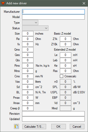
Entering fundamental T/S-parameters Re, Rms, Mms, Cms, Sd and BL first and let program calculate fs,
Qms, Qes, Qes and Vas (with c=344.0 m/s, ρ=1.194 kg/m3) is recommended, but not required.
You can enter Qms instead of Rms, Qes instead of BL , Vas or fs and Mms instead of Cms, Cms or Vas and fs instead of Mms.
Program calculates missing parameters (value=0) when OK button is pressed.
See tooltip of OK button for more information.
Pmax >0 W is required for maximum SPL trace (except for PR).
Xmax/Xsus >0 mm is required for maximum excursion trace.
Enter something smart if not known.
Check Crosscalc to update other parameters while one parameter is adjusted.
Radiators are simulated with Knudsen LOG model if Creep β > 0.
n0, SPL, USPL, EBP and Vd are calculated for information only.
Parameters are also possible to import with Import button or by Drag & Drop to 'Add new driver' window. Supported file formats are: VituixCAD .vxd, WinISD .wdr, Basta! .bastaelement, Hornresp .txt, SpeakerSim .sdrv and Speakerbench .json.
Parameters in xml format or measured and calculated with CLIO, LIMP, REW or Speakerbench summary table are possible to paste with Paste button.
Message is shown if something is missing or not parsed.

Thiele/Small parameters can be calculated with added mass or sealed box method by two impedance measurements and few known parameters. Calculation window opens with Calculate T/S... button.
Local driver database is saved automatically after driver is added or modified. Manual saving with Save Driver button or Save as... command in Database menu is required after Delete rows, Duplicate rows and Update database commands. Back-up local databases regularly.
Driver database is simple tab-delimited text file by default.
Initial/default database after installation is \Users\Public\Documents\VituixCAD\Enclosure\VituixCAD_Drivers.txt.
Database can also be XML file with either .vxd or .xml extension.
Note! It's highly recommended to use this default database only to maintain links between enclosure projects (.vxe) and drivers because
enclosure projects do not include T/S parameters. Just a link including pathname of local driver database (or online), driver manufacturer and model.
If necessary, user can create and maintain several local databases in different folders/servers via Database menu:
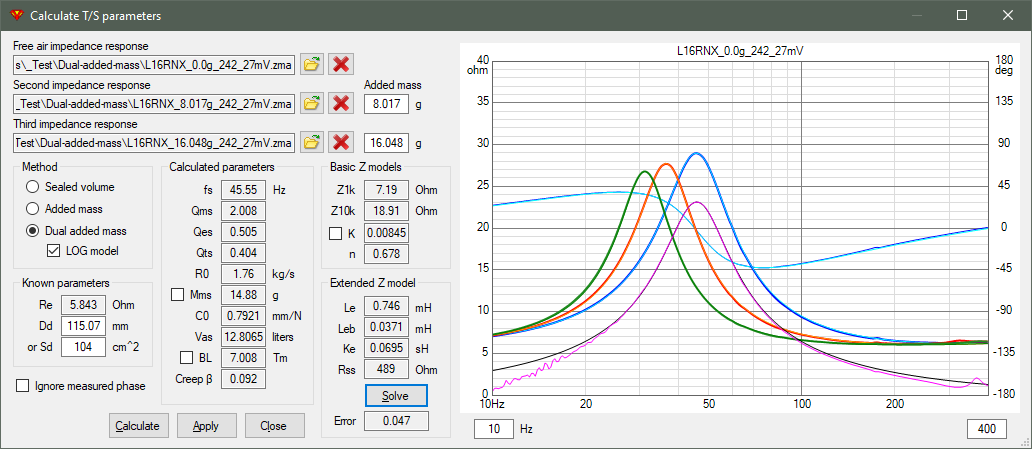
Required parameters for all calculation methods are driver's Dd [mm] or Sd [cm2] and free air impedance response measurement.
Re [Ohm] and second impedance response measured in undamped sealed enclosure with known volume are needed for Sealed volume method.
Re [Ohm] and second impedance response measured with known added mass are needed for Added mass method. Added mass ca. half of expected Mms.
Second and third impedance responses measured with known added mass are needed for Dual added mass method.
First added mass ca.
half of expected Mms, and second added mass ca.
expected Mms.
Check LOG model to calculate with frequency-dependent suspension compliance.
Extracted parameters are R0, Mms, C0 and Creep β.
Transfer function of fitted/simulated motional impedance:
Zem = Bl2 / (R0 + s * Mms + 1 / s / C0 / (1 + β * ln(1 + ω0 / s))), where ω0 = 3*pi*fs
References:
[1] J. Candy and C. Futtrup, "An Added-Mass Measurement Technique for Transducer Parameter Estimation"
[2] H. Hiebel, "Suspension Creep Models for Miniature Loudspeakers"
[3] M. H. Knudsen and J. Grue Jensen, "Low-Frequency Loudspeaker Models That Include Suspension Creep"
[4] https://speakerbench.com
Measure and load impedance response(s). Check Ignore measured phase if phase response is not reliable. Measure Re if needed and Dd if Sd is not known. Enter parameters and added mass [g] or sealed box volume [liters] to text boxes. Check Mms or BL if value is trusted and second impedance response measurement is not available. Press Calculate. Results are visible in Calculated parameters and Z model groups. Basic Z model parameters Z1k and Z10k, and Extended Z model parameters Le, Leb, Ke and Rss are detected from free air impedance response. Also Re is calculated with Dual added mass method. Leach Z model parameters K and n are detected from free air impedance response, and simulated Z response is visible in chart if K is checked. See tooltip of curves for more information.
Results can be accepted to previous Edit parameters/Add new driver window with Apply button.
Enclosure tool can use two different impedance models:
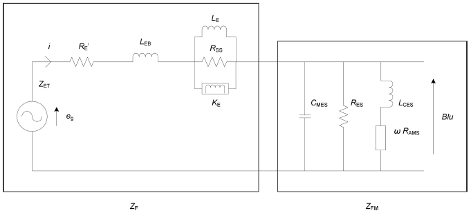
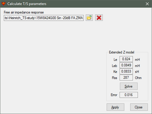
Voice coil inductance (with losses) is included in frequency response calculation by checking Show effect of inductance in context menu of SPL chart.

Local driver database can be updated with data on the clipboard or local file or online database @kimmosaunisto.net. Data format can be either xml or tab delimited text. Order and amount of columns in the source data and destination (local) database must match if the source data is not xml and does not have header line with parameter names. Column match should be verified especially with tab delimited text data on the clipboard. Local files and online database usually have header line or xml elements so the values are copied to correct fields regardless of column order.
Update database window opens via context menu of driver grid.
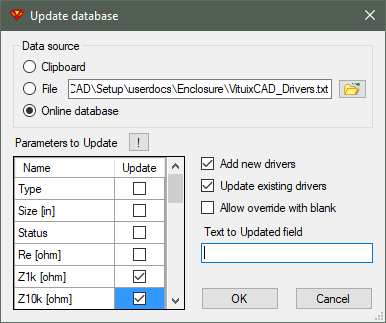
Select data source: clipboard, text/xml file or online database.
Drivers whose Manufacturer and Model are not found in the local database are added by checking Add new drivers.
Drivers whose Manufacturer and Model are found in the local database are updated by checking Update existing drivers. Select parameters to update from the list. Selections are inverted with [!] button. Allow override with blank enables replacing of existing value with blank. Otherwise blank value in the source data won't override existing non-blank value.
Text to Updated field overrides existing text. Text in the source data is copied if text box is left empty.
Drop down menu provides selection for amount of drivers. If more than one driver is selected, radio buttons on the right control how drivers are connected.
Number of drivers; 1, 2, 3, 4, 6, 8, 9 or 12 pcs, or pairs in isobaric configuration
Electrical connection; series, parallel, 2 || 2 ..., 3 || 3 ...
If Isobaric is checked, each driver in simulation is combination of two drivers mechanically in isobaric configuration. Isobaric pairs are connected electrically in series if series is checked. Otherwise pairs are corrected in parallel.
Extra mass per driver [g] can be used to simulate increase of Mms, which reduces fs and sensitivity of the driver. Mass is reset to zero grams by double-clicking 'Extra mass' label.
Amplifier's output signal as voltage U[V] or power P[W] to Re is common for all drivers. Voltage or power can be changed from default value to simulate cone excursion and vent air velocity with higher electrical power. Default signal (2.83 V or 1.0 W) is restored by double-clicking unit label.
Manufacturer and Model of previously selected driver is visible in text box. Volume excursion capacity Sd*Xmax*N is shown in Vd [cm3] field.
Radiator types supported by Enclosure tool:
Infinite baffle
|
Closed
|
Bass reflex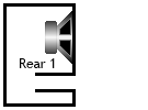
|
Double tuned reflex
|
|
Passive radiator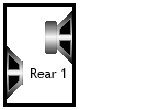
|
Band pass type 1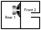
|
Band pass type 1P
|
Band pass type 2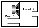
|
Band pass type 3
|

Closed box is aligned by selecting or entering Qtc.
Optional high alarm limit for non-linearity [% on Xmax] due to air compression is available.
Box volume is limited and requested Qtc is not produced if alarm limit is exceeded (red text).
Increase limit % until red color disappears to get requested Qtc if you don't care about compression distortion.
Distortion is calculated with 1.4 * Sd * Xmax / Vb * 100%.
Alignment is done with very basic formula: Vb = Vas / ((Qtc/Qts)^2-1).
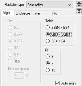
Bass reflex is aligned with SBB4/BB4, QB3/SQB3 or SC4/C4 table with Ql 3, 7 or 15 by Thiele, Hoge and Bullock, or
Quasi-Chebyshev (QC) table with 0.5 dB ripple and Ql=15 by L. Risbo.
See Speaker Box Alignments from Numerical Optimization - The Quasi-Chebyshev Alignment
Auto align executes alignment with entered parameters when driver or driver configuration or radiator type is changed.

Single cabinet impact response is possible to include in full space simulation shown in SPL graph (brown).
Load simulated baffle response by clicking Open button  ,
and enable it by checking Diffraction response.
,
and enable it by checking Diffraction response.
Diffraction simulator is executed by clicking Baffle step button  .
.
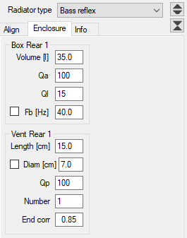
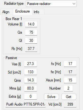
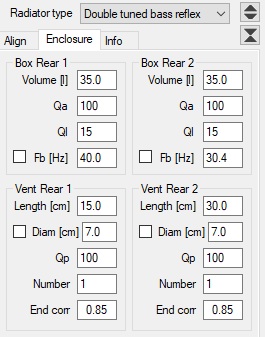
Adjustable box and vent parameters vary depending on chosen radiator type.
Adjustable box parameters: Volume [l], Qa, Ql, Fb [Hz]. Box resonance frequency Fb [Hz] is calculated read-only if box is not vented.
Adjustable vent parameters: Length [cm], Diameter [cm], Qp, Number, Total end correction; 0.60 - 2.40.
Fb [Hz] can be locked for vented box with checkbox: Vent Diam/Area is calculated if Length is modified. Vent Length is calculated if Volume, Fb, Diam/Area, Number of vents or End corr is modified. Table alignment unchecks 'Lock Fb' of Box Rear 1.
Get button reads passive radiator parameters from current row of driver database. Normal driver with motor is also possible passive radiator.
Manufacturer and Model of previously selected passive radiator is visible in text box. Volume excursion capacity Sd*Xmax*N is shown in Vd [cm3] field.
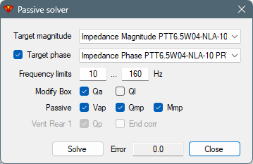
Some parameters of passive/vented radiators can be specified by comparing simulated impedance response to impedance response measured from known test system.
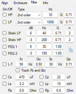
Filter tab enables adding max. six active filter stages, L+C+R in series with the driver(s) and L+C+R in parallel with the driver(s):
Note! Filter components are not included in impedance response export.
Stages are enabled (not shorted) with On/Off checkboxes. Transfer functions are calculated using DSP settings in the main program. Transfer function magnitude with filter blocks is shown in Group delay chart with dB scale (right).
Stages can be copied to clipboard with Copy button, and pasted to crossover in the main program. All twelve stages are copied if any block is enabled or Rs > 0. Disabled blocks/components are copied as shorted. Parallel L+C+R branch is set to open if all its components are disabled.
Filter settings are saved to enclosure project file (.vxe) only. Not to user config for the next session.
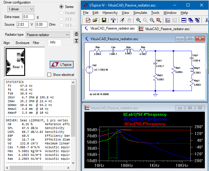
Info tab shows enclosure image, calculated acoustical parameters of driver, boxes and ports. Optional display of electrical equivalent values is available. Info tab also lists statistics: f-3dB, f-6dB, f-10dB, min. impedance, max. impedance, max. group delay, max. excursion of cone and passive radiator and max. air velocity of vents.
Optional execution of external LTspice circuit simulator is available. Acoustical parameters of driver and enclosure are passed into LTspice. Path for LTspice executable needs to be defined in Options window.
Note! Effect of voice coil inductance is not shown in SPL curve.
Total SPL to half space and impedance response can be exported if you choose to use them in simulating loudspeaker driver instead of acoustic and electrical measurements. Impedance response (txt/zma) is routed to driver selected in Drivers tab in the main program by checking Feed before exporting.
Enclosure project is saved with Save Project button, and opened with Open Project button or Enclosure project table (arrow down button).
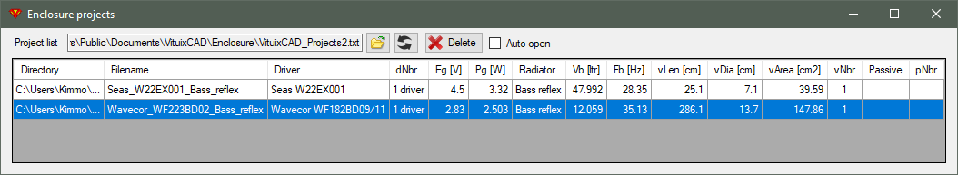
Enclosure project list can be changed with Open button. Default list file is \Users\Public\Documents\VituixCAD\Enclosure\VituixCAD_Projects.txt.
Project list and data in vxe files is reloaded to the table with Refresh button. Selected rows are deleted with Delete button. Note! Enclosure project files (vxe) are not deleted. Projects open while browsing the list by checking Auto open. Project opens and list window closes by double-clicking row also when Auto open is unchecked.
Frequency axis limits can be adjusted with text boxes in the bottom. Every graph can be zoomed to full size and back to dashboard by double clicking in middle area of particular graph. Color coding of traces is defined below dashboard. Dashboard of enclosure tool includes following graphs:
See tooltips or Traces... to identify curves. See Chart overlays.
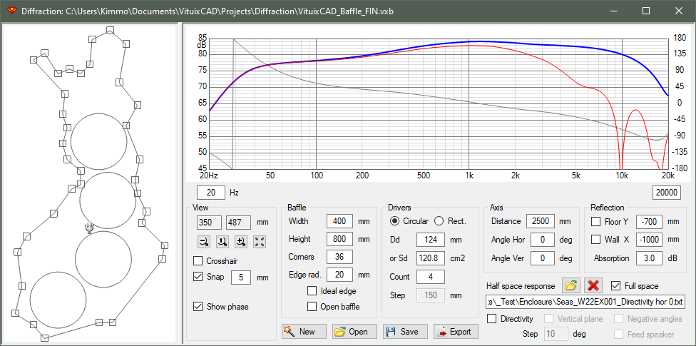
Diffraction simulator calculates cabinet impact or full space frequency response of driver(s) in a baffle. Simulation is based on simple ray theory: each driver is a point source sending 72 rays towards baffle edges with fixed 5 deg steps. Path lengths of shortest 1st order diffractions are calculated and summed with delay i.e. phase information in a listening point. Magnitude of diffracted rays is frequency dependent. Weighting factors are calculated from radiator dimensions and edge radius. Maximum amount of corners is 36, and minimum is 3. Baffle can contain up to 50 drivers with equal dimensions. Simplified room response with floor and side wall reflections is available.
Start baffle designing by entering main dimensions; width, height and number of corners. Select driver shape; circular or rectangular. Enter effective diameter Dd or area Sd for circular or width and height for rectangular, number of drivers and Step which is vertical distance between drivers (if more than one). Press New button to create initial shape with drivers and mic in the drawing area.
Adding and deleting of corners and drivers is available via context menu. Corner is added in the cursor position, but you may need to rotate two corners to get new one to correct position. Driver is added in the cursor position.
Zooming Out, 1, In and Fit are available via zoom buttons  .
You can pan baffle image by dragging when nothing is selected (blank area clicked).
Unit of location coordinates is millimeter.
Zoom 1 equals 1px=1mm.
Origin (0, 0) is initially in the bottom left corner.
Origin can be moved to cursor position by clicking left button when Ctrl key is pressed.
If corner, driver or microphone is selected, origin moves to the center point of selection.
'Set origin (0,0)' command is available also in context menu.
.
You can pan baffle image by dragging when nothing is selected (blank area clicked).
Unit of location coordinates is millimeter.
Zoom 1 equals 1px=1mm.
Origin (0, 0) is initially in the bottom left corner.
Origin can be moved to cursor position by clicking left button when Ctrl key is pressed.
If corner, driver or microphone is selected, origin moves to the center point of selection.
'Set origin (0,0)' command is available also in context menu.
Half space frequency response of driver can be loaded for full space response simulation. Enable full space view and export by checking Full space. Y-scale is adjusted automatically.
Check Open baffle for dipole speaker with thin I-baffle.
Individual objects; corners, drivers and microphone are selected by clicking left button above the image. Selected object is highlighted and location (X, Y) is visible in View group. Location can be adjusted by dragging or entering coordinates or pressing arrow keys in the text boxes. Baffle width and height are updated to text boxes after corner is moved with mouse or arrow keys or text box. Snap setting restricts object movement to intervals specified with the text box. Snap mode is activated by a checkbox. Object is moving orthogonally if Shift key is pressed while dragging. Baffle width and height can be adjusted with text boxes after baffle is created with New button. Movement of corners is relative to selected origin. Crosshair cursor helps object aligning. Cabinet impact response graph is updated while adjusting.
Remove selection (deselect) by clicking blank area. Coordinates of mouse cursor are shown as long as nothing is selected.
Edge radius and Driver Dd or Sd, Width and Height can be adjusted after project initialization by entering value or pressing up/down keys in the text boxes. Drawing and cabinet impact response graph are updated while adjusting.
This is a simple emulation for directivity of a waveguide. Emulation does not include change in efficiency and on-axis SPL. There is no response boost (and anyhing for impedance) so result cannot be used for designing equalization. Actual waveguide/horn simulation would be much more complicate requiring all dimensions, shape of cross-section(s) and driver parameters.
Emulation is activated with Enable checkbox in 'Waveguide mimic' group.
A circle in green dashed line is drawn outside the driver(s) when emulation has been enabled.
Frequency where directivity starts is adjusted with Cutoff textbox in Hz.
Change in directivity as a function of frequency is adjusted with Slope text box in dB/oct.
Value to be adjusted is slope of off-axis response to 90 degrees in half space (infinite baffle without directivity due to baffle edges).
Range is from -0.1 to -6.0 dB/oct.
Root response for emulated off-axis responses is transfer function of the 1st order low-pass filter.
That is manipulated with Slope parameter and direction (angle) from the driver to virtual mic/listening point.
Waveguide is assumed to be circular.
Directivity calculation of the driver (as an ideal piston) is limited between -50 and +50 degrees i.e. opening angle of the throat is assumed to be ca. 100 degrees.
Microphone symbol represents listening point at Axis Distance. Enter 5000-30000 mm for far field simulation to get full baffle loss. Baffle can be rotated horizontally and vertically by entering Angle Hor or Angle Ver, or pressing up/down keys in the text boxes. Rotation origin is perpendicular point of microphone on (unrotated) baffle surface. Horizontal rotation of baffle is positive to counter-clockwise from top view. Vertical rotation of baffle is positive to face up. Sign of rotation angles are changed while directivity export for compatibility with measurement data.
Check Floor and enter floor elevation in mm to include floor bounce in frequency response. Side wall reflection is included by checking Wall. Negative X coordinate locates wall on the left side. Enter absorption within 0...20 dB to reduce amplitude of boundary reflections.
Save baffle project by pressing Save button. File extension is .vxb, but it's human-readable xml file containing main dimensions and location of corners and drivers. You can print the file for helping final enclosure design.
Open existing baffle project by pressing Open button.
Export simulated Cabinet impact response or full space frequency response shown in the graph by pressing Export button.
You can also export off-axis responses with adjustable steps (1-45 deg) by checking Directivity. Responses to positive angles in vertical plane are exported by checking Vertical plane. Responses to negative angles are exported by checking Negative angles. Responses are routed for currently selected driver in the main program by checking Feed speaker before exporting. Enter root file name for responses. Program extends file name with horizontal/vertical keyword and angle, using coding defined in Options window.
See tooltips or Traces... to identify curves. See Chart overlays.
Note!

Conversion tool imports multiple impulse response (IR) files and converts to frequency response (FR) files. It is recommended that all files in the list are measured with common parameters and settings: rotation center, distance, level, signal type, sampling rate, MLS sequence length etc.
Load impulse responses to file list with Open button or Drag&Drop. More measurement files can be added to the list by pressing Shift key while dropping or clicking Open button in file selection dialog box. Supported IR file formats are ARTA .pir, CLIO Standard/QC .mls/mlsi (4.x, 6.x, 7.x), CLIO Pocket .crp, WAV mono/stereo (16-bit PCM, 24-bit PCM, 32-bit PCM, 32-bit IEEE, 64-bit PCM, 64-bit IEEE) and MLSSA/SE .txt. Wav files may contain proprietary/custom chunks such as FLLR or APx5. Program asks sample rate if .txt file does not have valid MLSSA ASCII header. Values are read from column 2 if measurement .txt file contains more than one data column. Combo boxes on the right show sample rate in Hz and scale type: Pascal, Ohm, Volt of currently selected IR file. 'Skip samples' text box enables ignoring extra samples in the beginning of impulse response file (added by measurement program). For example ARTA adds 300 samples to pir files and Praxis about 1ms x sample rate to exported wav/txt files. Check Invert to change polarity of impulse response. ETC curve can be smoothed by 0-32 samples with ETC smooth text box.
Selected file is visualized in the graphs.
Click Far 1 button to set default values for the 1st far field export (tweeter's) while on-axis response is selected. Following far field exports (mids and woofers) of the same speaker should use the same settings except length of right window which is adjusted for each driver by the first undamped boundary reflection.
Click Near button to set default values for near field export while response of mid or woofer cone is selected. All near field responses can be exported at once.
Click Z/U button to set default values for impedance, voltage and acceleration export.
Impulse responses are possible to save as space delimited text, csv or MLSSA text files to selected Directory by pressing small export button on the left size of Far 1 button.
FFT session is possible to save as vxf-file with 'Save session' button, and load with 'Open session' button. IR file list and FFT analysis, Output and graph settings are saved to session file.
Impulse response is multiplied by window function (sample by sample) before conversion to frequency domain with Fast Fourier Transform (FFT). Typical purpose of window function is to crop room reflections from measurement data. Window function could have one or two sides. Left side is activated with Left window checkbox. Maximum point of window function and phase response of exported frequency responses are set with Reference time. Reference time is typically set to the first sharp and high (positive) peak of impulse response to produce close to minimum phase response at high frequencies. Get button locates reference time to the highest absolute peak of impulse response. Manual fine tuning may be needed. Name of Reference time will change to Start time if Left window is disabled. Right window is 'main gate' for measurement data after Reference/Start time. Endpoint of right window is typically set in the beginning of the first stong boundary reflection (not diffraction).
Available Window functions are Rectangular, Bartlett, Blackman, Blackman-Harris, Blackman-Nuttall, Cosine 0.50/0.75/1.0, Hamming, Hanning, Nuttall and Tukey 0.25/0.50/0.75. Flat top functions Rectangular and Tukey allow some movement or location differences or timing differences of measured objects so that impulse does not attenuate too much or flow totally out of time window. Recommended functions for driver measurements with rotation table is Tukey 0.50.
Side effect of rectangular right window could be HF artefacts/errors in frequency response. Hanning function is not recommended either, but could be usable if timing and location of measured objects are constant and response does not have much resonances i.e. possible variations in IR are small or very close to first peak.
Reference time and length of time windows are adjusted by mouse via impulse response graph, or in milliseconds (ms) or samples (smp) or millimeters (mm) with text boxes in FFT analysis group.
FFT length could change automatically while adusting length of time windows to ensure that whole time window fits into FFT buffer. FFT length is possible to change after window length adjustments. Extending may be needed to increase accuracy/resolution at low frequencies.
Effect of possible DC voltage in the input or ouput of sound card can be reduced by checking DC offset. Average IR level before time window (max. 270 samples) is calculated and subtracted from all IR samples.
Boundaries of displayed and exported frequency responses are adjusted with Frequency range text boxes. Widest possible range is from 5 Hz to 40 kHz or sample rate / 2 (Nyquist frequency) which one is lower. Low frequencies may need cropping due to noise or other inaccuracies if measured object does not pass low frequencies. Highest frequencies may need cropping due to limits of measurement system. For example if sweep stops shortly before sample rate / 2.
Frequency response Smoothing of 1/24, 1/12, 1/6 or 1/3 octs. is available. Smoothing function is 6th order Butterworth band-pass, slopes truncated at -20 dB.
Calibration of sound pressure (in Pa) measurement is enabled with Calibration checkbox. Calibration file is selected into text box with Open button or Drag&Drop. Minimum phase extraction should be applied with Minimum phase checkbox if calibration file does not include phase information. Calibration does not apply if unit of IR measurement is Ohm.
Target folder for frequency response files is selected into Directory text box.
Warning! Existing output files will be overwritten without warning. Select different output directory if both impulse and frequency response files are .txt, or export frequency responses as .frd files.
Magnitude can be scaled with Scale text box: in dB for dBSPL and dBV, and multiplier for Ohm. Metadata can be added to output file by checking Info header.
File format and extension is selected with File format list box. ZMA is selected if unit of impulse response is Ohm. Magnitude unit is dBV if unit of impulse response is Volt. TXT produces 3-column space delimited text file with header line. FRD and ZMA produce 3-column tab delimited text file without header line. LMS produces 3-column comma delimited text file without header line. WAV exports 32-bit IEEE mono as time-windowed and scaled impulse response. Smoothing is not supported with WAV export.
Full resolution checkbox exports unsmoothed high resolution frequency responses. Frequency step is constant sample rate / FFT length allowing long excess delay without wrapping errors in phase response.
Warning! Use short FFT to avoid huge file size and slow processing.
Output files are created with Export button. Only the selected response is exported when Ctrl key is pressed while clicking Export button. Responses are loaded for currently selected driver in the main program if Feed speaker is checked.
Impulse graph contains impulse response (blue), optional impulse envelope (ETC, dark green), impulse dBFS (dark cyan) and step response (orange red) and overlays, window function (gray), three cursors: Left window start (orange), Reference/Start time (magenta) and Right window stop (red). Cursor legend shows time (ms), impulse magnitude (Pa/Ohm/Volt) and envelope/impulse dB at cross cursor position if cursor dragging is not on. While dragging with left button down, cursor legend shows magnitude of impulse (Pa/Ohm/Volt) at cursor time (ms) and distance to Reference (mm).
Magnitude and time scales are adjusted manually with Expand and Compress buttons.
Press Ctrl key to expand/compress dB span of impulse graph.
Time scale is panned manually with Left and Right buttons.
Auto buttons scale magnitude and time axes automatically.
Magnitude axis is scaled to absolute maximum and time axis to show whole time window - not impulse peak if it's not inside time window.
See tooltips or Traces... to identify curves. See Chart overlays.
Frequency response graph shows magnitude (blue), phase in degrees (gray), optional minimum phase response (lime),
excess phase response (steel blue), overlays and 'gating frequency' with vertical line at 1.0/right_window (magenta).
Result below gating frequency could be unreliable and too smoothed, but it depends on shape of impulse response and selected window function.
For example perfectly flat system produces correct result also with very short time window.
See tooltips or Traces... to identify curves. See Chart overlays.
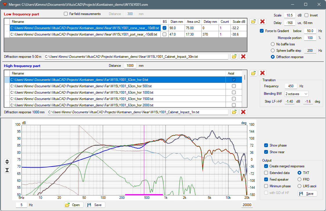
Merger tool merges frequency responses using two separate sections: Low frequency part and High frequency part. Low frequency responses can be either far field (4pi) measurements or near field (2pi) measurements with baffle simulation and measured or textbook directivity. Graph shows preview of low frequency part (red), high frequency part (blue), merged response (WindowFrame) and optionally phase (gray) and individual near field LF responses (green). Graph cursor (magenta) controls transition frequency and shows also blending range.
See tooltips or Traces... to identify curves. See Chart overlays.
Merger tool merges near field measurements with diffraction simulation, measured directivity and optional textbook directivity to time-windowed far field measurements.
Uncheck Far field measurements.
Near field frequency responses are added by clicking folder button on the right or dropping files into the list.
You can have multiple responses, usually near field of cone(s) and port(s) or passive radiator(s).
Check BS if the cone/port/passive is located on the front panel creating baffle step to on-axis direction.
Leave BS unchecked if cone/port/passive is located on the side, top, bottom or rear panel because there's no baffle step to on-axis.
Enter diameter [mm] or area [cm2] of radiating surface to enable automating scaling to far field and
directity simulation for ports/passives located on other than front panel.
Enter travel difference to active cone on the front panel at typical listening distance (2-4 m) on-axis to Delay [mm] field.
For instance, delay is ca. panel width / 2 + box depth if the port/passive radiator locates in the middle of rear panel.
Delay should normally be zero for active cones on the front panel.
Scaling can be adjusted with Diam [mm], Area [cm2] and Count of radiators or Scale [dB] in response rows, and
for total low frequency part via Scale or Distance text box by entering a value or by Up/Down keys.
'Force to Gradient' checkbox and 'Monopole portion' text box enable forcing ideal gradient directivity to near field LF responses
if directivity of far field HF responses is too unreliable at LF due to window function or measurement conditions,
and directivity at LF can be predicted without measurements.
Monopole portion values for known gradient radiators:
Omni 100 % (DI 0 dB), Cardioid 50 % (DI 4.8 dB), Super-cardioid 37 % (DI 5.7 dB), Hyper-cardioid 25 % (DI 6.0 dB), Dipole 0 % (DI 4.8 dB).
Directivity of far field HF responses is used at LF when 'Force to Gradient' is unchecked.
Highest frequency using ideal gradient pattern is adjusted with 'below Hz' text box.
Directivity is blended within ideal gradient range and transition frequency.
Narrowest blending range is one octave.
For baffle diffraction there are three options available: No baffle loss, Sphere baffle step (adjustable nominal frequency) or Diffraction response. 'Diffraction response 5-30 m' can be selected by clicking folder button or dropping file into text box. Baffle effect response simulated to the longest ever possible listening distance is selected into this text box. Response type must be 'baffle step' i.e. scaling 0...+6 dB.
Low frequency response list must have equal off-axis angles (with the same angle coding in filenames) with high frequency response list. Otherwise LF and HF responses cannot be paired.
Check Far field measurements. Far field frequency responses are added by clicking folder button on the right or dropping files into list. Enter Distance of low frequency and high frequency measurements to calculate scaling of LF responses automatically. Scaling can be adjusted via Scale text box by entering a value or by Up/Down keys.
Far field measurements can be added by clicking folder button or dropping files into list. On-axis response is selected by checking 'On-axis' column in response file list. Default on-axis response is 0 degrees in horizontal plane. Merged responses (graph below High frequency part) to particular angle can be previewed by clicking corresponding file from HF response list.
Enter actual measurement distance in mm to Distance text box.
Optional 'Diffraction response X mm' can be selected by clicking folder button or dropping file into text box. Baffle effect response simulated to actual measurement distance of far field High frequency responses is selected into this text box. Response type must be 'baffle step' i.e. scaling 0...+6 dB.
Transition from low frequency to high frequency part can be adjusted manually via Frequency text box, graph cursor or Up/Down keys.
Warning is given with red background color if transition frequency exceeds maximum near field frequency of the largest low frequency radiator. fNFmax = c/pi/Dd (c = 344.0 m/s).
Magnitude and phase blending range between low and high frequency parts can be selected from list box: none, 1/2, 1, 2, 3 or 4 octaves.
Delay of low frequency part is calculated automatically on transition frequency change but can be adjusted manually.
Choose which items you want to output. Create merged responses will combine low frequency and high frequency responses into individual response files. Extended data will combine LF and HF responses into a single file, having LspCAD 6 extended data format. Merged responses are routed to main program for currently selected driver in Drivers tab by checking Feed speaker before saving.
Output response can be limited within visible frequency range by checking 'Visible frequency range only'. Normally it should be unchecked to avoid forced extrapolation which is never accurate. Limiting can improve e.g. impulse response graph in case LF (or HF) part of merged response is inaccurate due low SNR at infra frequencies such as <= self-resonance of passive radiator.
Merged responses are exported as minimum-phase by checking Minimum phase. Measured and entered delays are lost and all responses at all frequencies are normalized to the same acoustic center = 0 mm. Color of merged phase response is lime in the chart.
Excess group delay of HF response at transition frequency x 1.4 is added to merged minimum phase response by checking with GD of HF. This option saves measured delay (at transition frequency x 1.4) and delay adjusted by user.
Minimum phase options may be needed if measured far field HF responses are not minimum-phase at transition frequency, though radiator is actually minimum-phase. Significant error is possible with some measurement programs if IR time window is short. Forcing to calculated minimum phase is not recommended if responses are measured with dual channel gear and phase error at transition frequency is just few degrees.
Output file format is selected with TXT, FRD and LMS ascii radio buttons. Result files are saved to destination directory selected with browse folder dialog.
Merger project can be saved with Save button in the bottom left corner. File extension is vxm, internally XML.
Saved merger project can be opened with Open button or dropping vxm-file into Merger tool window.
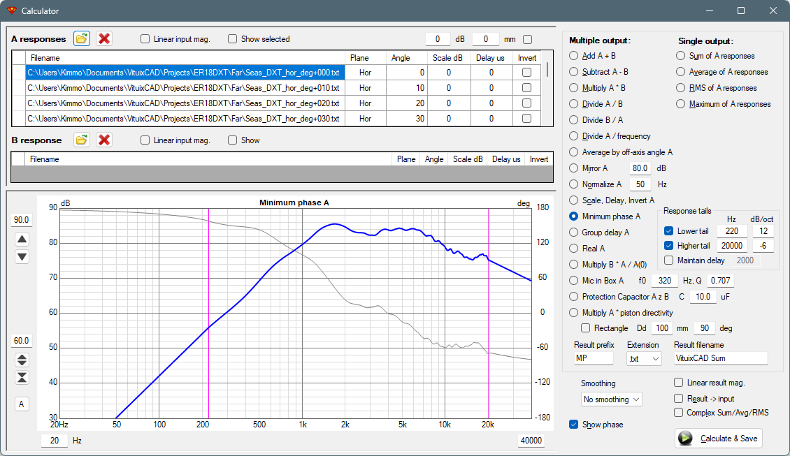
Calculator tool is a generic math tool for frequency response file processing. Most of the math skills required for speaker simulation are included in Enclosure, Merger and Diffraction tools and crossover simulator. Calculator tool provides some additional functions and flexibility to process calibration files, preprocess measurements before simulation or analyze complete speaker or a single driver.
Primary response list is 'A responses'. It accepts multiple responses. 'B response' is single response.
Add response files by clicking folder button or dropping files into list. Multiple file selection with Open dialog is enabled. Delete button clears whole response list. Uncheck Linear input mag if magnitude is in dB value in the response files. Check Linear input mag for impedance, pressure or voltage responses where magnitude is not in dB value. Phase angle unit should be degrees. Calculator wraps phase automatically within -180...+180 deg. All loaded files are processed.
Manual scaling, timing and polarity inversion is available for each response. Simultaneous scaling/timing/inversion of all responses is available above response list. Phase angle in the filename is detected and visible after filename. It is needed for directivity and power response calculation. See Options for more information.
Functions for each input response A, producing multiple result responses:
Responses A added by response B.
Default result filename prefix is AddAB.
Responses A subtracted by response B.
Default result filename prefix is SubAB.
Responses A are multiplied by response B.
Default result filename prefix is MulAB.
Responses A are divided by response B.
Default result filename prefix is DivAB.
Response B is divided by responses A.
Default result filename prefix is DivBA.
Responses A magnitude is divided by frequency.
Default result filename prefix is DivAf.
Calculates average of the same plane and angle.
This is handy when crossover is designed with several driver samples having some real life tolerances i.e. differences in frequency responses.
All measurements of drives samples are loaded to A responses.
Program sorts response list by Plane, Angle and Filename, and calculates and exports average of each off-axis group to response files which can be loaded to Drivers tab in the main program.
Result's magnitude is arithmetic mean of magnitudes to avoid magnitude drop due to possible delay differences between acoustical measurements to the same off-axis direction.
Result's phase angle is vector sum to avoid phase unwrapping (which would be required for arithmetic mean).
'Complex Sum/Avg/RMS' is unchecked and disabled to force previous settings.
Note! 'Angle parsing from filename' settings in Options must match with loaded frequency response filenames to get correct values to Plane and Angle columns.
Default result filename prefix is AvgByDir, followed by plane and off-axis angle of the group. Angle coding uses current 'Angle parsing from filename' settings in Options (so you can also change angle coding e.g. from 3D balloon to generic 2D).
Responses A mirroring aka vertical flipping over entered dB value.
Default result filename prefix is Mir.
Responses A normalizing to magnitude of the first response A at entered frequency.
Default result filename prefix is Norm.
No calculation - just responses A magnitude scaling, time shifting and polarity inversion.
Default result filename prefix is Sca.
Responses A converted to minimum-phase. Response tails below 5 Hz and above 40 kHz are estimated by the first and last 1/2 octaves. Response tails can also be specified manually by checking Lower tail and Higher tail and entering cropping frequency and slope in dB/oct in Response tails group.
Excess group delay can be added to maintain delay of original response. Check Maintain delay and enter frequency where phase shift should be equal to original response.
Default result filename prefix is MP.
Responses A group delay in milliseconds.
Default result filename prefix is GD.
Responses A converted to real: phase angle is set to 0 deg or -180 deg if Invert is checked.
Default result filename prefix is Re.
Creates off-axis responses for measured or captured on-axis response B with directivity information in responses A. Directivity data can be simulated with Diffraction tool or compatible set of far field measurements. Response A to 0 degrees is reference in directivity calculation.
Default result filename prefix is MulBdirA.
Responses A are multiplied by 2nd order high-pass and polarity inverted. Corner frequency and Q-factor are specified with following f0 and Q text boxes.
Default result filename prefix is Mib.
Function calculates correction to response measured with Microphone-in-Box technique, or any other response including effect of close to ideal room gain at low frequencies.
For more information: Measuring Loudspeaker Low-Frequency Response.
Compensates effect of protection capacitor in series with driver while frequency response measurements with semi- or full dual channel mode i.e. reference channel is connected to output of sound card or power amplifier. Not between protection capacitor and driver!
Load frequency responses (txt/frd) to A and impedance response (txt/zma) to B. Verify that Linear input mag A and Linear result mag are unchecked, and Linear input mag B is checked. Enter series capacitance to C/uF text box.
Default result filename prefix is Uncap.
Responses A multiplied by piston directivity. Calculation parameters are piston diameter for circular or width for rectangular radiator, and off-axis angle in degrees. Off-axis angle coded in filename in response list A is applied if 0 degrees is entered. Directivity function for circular radiator is 2*J1(k*a*sin(angle))/(k*a*sin(angle)), where J1(x) is 1st order Bessel function of first kind, k=wave number and a=radius. Directivity function for rectangular radiator is Sinc(k*x*sin(angle)), where x is width. Result response is minimum-phase.
Default result filename prefix is Pis.
Functions for multiple input responses, producing single result response:
= A0 + A1 + A2 + ...
Default result filename is VituixCAD Sum.
= (A0 + A1 + A2 + ...) / N
Default result filename is VituixCAD Avg.
= SQRT((A02 + A12 + A22 + ...) / N)
RMS is alternative for simple average (arithmetic mean). Square scales single magnitude value for area or power, for example from sound pressure to intensity. See Complex calculation.
Default result filename is VituixCAD RMS.
Searches maximum magnitude from responses (A) for each frequency point. Phase angle of result response is taken from selected row.
Default result filename is VituixCAD Max.
Result filename extension is selected with list box. Available options are .txt, .frd, .cal, .mic, .lms, .etx and .zma
Complex Sum/Avg/RMS should be checked in order to calculate complex vector sum, average or RMS with phase angle information. Complex calculation is sensitive to phase angle; sum of two equal magnitudes with opposite polarity = 0. This is default option giving correct results with frequency responses.
Absolute magnitudes are summed if Complex calculation is not checked. This option is useful if phase information is too random or nonsymmetrical (like with multiple room responses) causing steep magnitude dips in result response. Phase angle of result response is calculated with complex numbers anyway, but minimum phase features are not completely maintained.
Smoothing options are 1/1, 1/2, 1/3, 1/6, 1/12 octaves or none. Smoothing function is 6th order Butterworth band-pass, slopes truncated at -20 dB.
Result files can be recycled to input responses by checking Result -> input. Multiple result files are recycled to responses A, and single result file to response B. This enables calculation sequences without manual loading of result files to input.
Result files are created by clicking Calculate & Save button. Files are saved to destination directory selected with browse folder dialog. Calculation to graph without result file creation is executed when response files are loaded or calculation formula is selected or smoothing or any other additional option is changed.
Result files saved as .cal or .mic are compressed by skipping frequency points where magnitude slope changes less than 0.12 dB/oct. At least one point per octave and first and last point are written though response is perfectly flat.
Enter title directly into graph for publishing of captured image.
Maximum and span of magnitude axis are adjusted by arrow buttons or entering value or Up/Down keys in the text boxes. Visible frequency range is also adjustable. Magnitude can be auto scaled by clicking A button. Scale of phase axis is constant -180...+180 deg.
Magnitude and phase of selected response A are shown by checking Show selected.
Magnitude and phase of response B is shown by checking Show.
See tooltips or Traces... to identify curves. See Chart overlays.

Calculates maximum length of time window (ms) without reflections. Enter shortest distance from driver to mic, from driver to floor and from mic to floor (mm). Calculates also path length of reflection (mm) and minimum frequency (Hz) with 1/1, 1/2 and 1/3 octs. resolution.
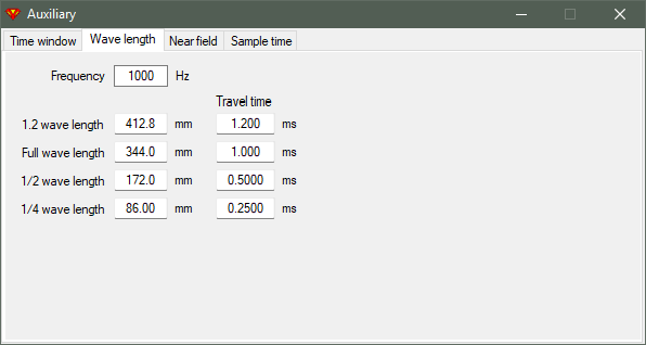
Calculates 1.2x or full or 1/2 or 1/4 wave length (mm) and sound travel time (ms) in air by frequency (Hz).
Enter 1.2x or full or 1/2 or 1/4 wave length to calculate frequency and travel time.
Enter travel time of full wave or fraction to calculate frequency and wave length.

Calculates maximum near field frequency (Hz) and maximum distance (mm) to microphone by effective piston diameter (Dd mm) or area (Sd cm2). This gives approximately -0.5 dB error at fNFmax in theory if mic is in the center point of ideal piston. In practice maximum applicable frequency is usually lower due to non-centered mic location and mechanical properties of the cone.
fNFmax = c/pi/Dd (c = 344.0 m/s)
Max. distance to mic is 5.5% of Dd.

Calculates time (µs) and distance in air (mm) for 1 and 2 and any number of samples by sample rate (Hz). You can also calculate number of samples and distance by time, or number of samples and time by distance.
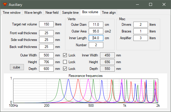
Calculates outer dimensions (mm) by net volume target (liters), wall thicknesses (mm) and internal volume losses due to vents, drivers, braces and amplifier box. You can lock one or two aor all outer dimensions. Target volume is recalculated if all outer dimensions are locked. Cube button resets shape to cubical. Graph shows frequencies of internal axial modes by width (red), height (green) and depth (blue) as well as open pipe resonances of vents (magenta).

Time align function can be used to specify delay/distance difference between acoustic centers of two drivers. Delay can be iterated manually with delay [µs] or distance [mm] text boxes, or with a solver. Three response measurements are needed. They should be measured at the same spot in the middle elevation of the drivers, or at normal listening distance and elevation if speaker will be designed with on-axis responses only. Two measurements from individual drivers and one measurement when both drivers are connected in parallel to power amplifier, maintaining supply voltage for individual drivers.
Load first driver response (usually mid-woofer) to LF measurement text box with Open button or Drag&Drop. Red curve is shown in graph. Check MP on the right if response is not minimum-phase i.e. excess group delay is not yet removed with measurement program or Minimum phase function in Calculator tool.
Load second driver response (usually tweeter) to HF measurement text box with Open button or Drag&Drop. Blue curve is shown in graph. Check MP if response is not yet minimum-phase.
Load sum response of drivers to Sum measurement text box with Open button or Drag&Drop. Magenta curve is shown in the graph. Sum measurement does not need minimum phase extraction, because it's phase response is irrelevant for this operation.
Adjust Frequency range limits which are also constraints for the solver. Exclude frequencies which are not valid for solving the delay.
Adjust delay in microseconds [µs] or distance in millimeters [mm] until Calculated Sum (green curve) is close or equal to Sum measurement. Scale Sum measurement either manually or by clicking dB label, if SPL at low frequencies is not equal to Calculated sum (green). Solver can be started with Solve LF delay button to seach minimum squared error between Sum measurement and Calculated Sum. Sometimes solver may need decent initial delay value to find correct local minimum. Error value is high with red background if solver did not find response match.
Difference in acoustic centers should be entered as a delay to Delay µs parameter in Drivers tab with unidirectional drivers such as closed or vented enclosures and horns. Not to Z mm coordinate of driver instance in crossover to avoid probable response summing error to off-axis >60 deg.
Difference in acoustic centers should be entered as a distance to Z mm coordinate of driver instance in crossover with dipole drivers to enable more accurate geometry simulation to off-axis >60 deg.
Note1: This method is not necessarily accurate due to subjective nature and limited radiator support of minimum phase extraction.
Note2: This method is not recommended for off-axis, power response and directivity index simulation because delay/distance difference between acoustic centers is not constant value to all directions 0...±180 deg with different radiator types such as domes, cones, horns etc. and enclosure types such as boxes and dipoles. Time align feature has been added to support at least simulation of on-axis and listening window responses. Simulation options are limited for users who don't have adequate measurement gear for accurate and stable timing measurements with dual or semi-dual channel connection and measurement mode.
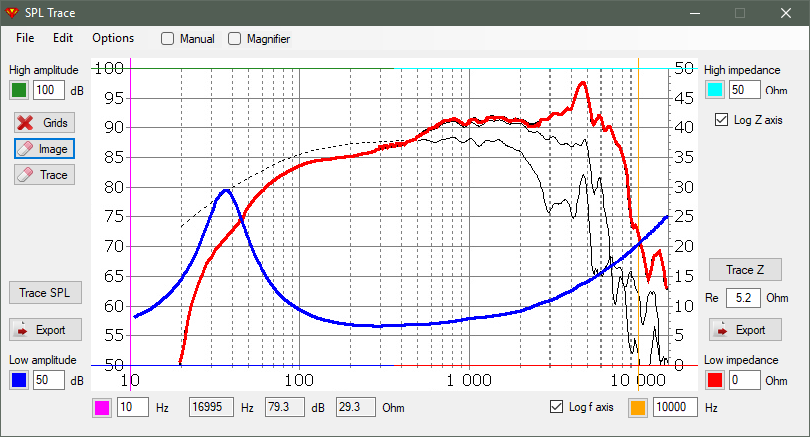
SPL Trace tool can capture frequency and impedance responses from bitmap loaded from file or pasted from the clipboard. Several image file types are supported such as png, jpg, bmp and gif. Some external tool or print screen is needed for copying bitmap to clipboard from datasheet (pdf) or web page. Snipping Tool installed in Windows 10 works fine.
Recommended size of bitmap is 800x400px or more to enable adequate resolution and accuracy. Bitmap is shown in SPL Trace window with original size or fitted smaller if needed.
Note! Dark background color of bitmap should be replaced with light with Edit -> Invert colors command.
Extracting of responses:
Traced sound pressure points can be copied to clipboard with Edit -> Copy raw SPL. Traced impedance points can be copied to clipboard with Edit -> Copy raw Z. Phase angle is zero and decimal symbol defined in Control panel.
Press Shift key while moving mouse above the image to open circular Magnifier of 400 %. Check Magnifier to show continuously. Pressing Shift key hides magnifier temporarily. Frame of the magnifier shows color at mouse cursor while tracing.
Captured curves can be shown with highlighted and partly transparent color by checking Options -> Green SPL, Cyan Z.
Needless to say, filters are the brain and heart of speakers. As music evolves over time - we accept the parameters of Time as Suprime (highest important) than the STATIONARY frequency response. This does not mean a limited and curved frequency response.
Proper full band signal reproduction requires all spectral components to be arranged with their exact amplitudes, which are constantly changing and are crucially dependent on the time domain.
The idea arose when as a musician (bass guitar) and as a sound director I listened to the general (mixed) sound from two-way and three-way speakers. There were no micro details, natural timbres, attack (increase) and decrease (fading reverberation) in time and space. There was no sense of a specific scene and no directives from individual instruments and vocals. The big ambition for me was after reading a study by R. Heiser and later Lipshitz, Vanderkooy, Kreskovsky. F.Brooke's articles "Le filtre ideal" in L'AUDIOPHILE was no small stimulus and last but not least. The Loudspeaker Cookbook by V. Dickason has been my desktop reading for many years. Of course - the biggest challenge was the "hidden" delays (resonances) of the filters, higher than the first order. This technology is very important, but it is not a wizard panacea for all other problems and omissions. We can not talk about good Timing - if there is a band with reverse polarity. But it is not superfluous to know - before measuring the impedances and frequency responses for the future project, an appropriate selection of speakers must be made, incl. preliminary solution for optimal shear frequencies. Ie - together with the choice we specify: The self resonance of each high frequency (of course and middle driver) must be one / two octaves farther (down) from the filter frequency. The rule is general alignment according to the quietest speaker. Ensuring flat (constant) impedance for each filter - too. Working with a simulation program is essential (help). Pre-planning the possibility for precise movement between the centers of the adjacent drivers (speakers) through separate enclosures (boxes) - mandatory. Precise observance of results (values) from the filters, including displacement (delay) - too.
If we get as close as possible to a better Step Response - this would be adequate to the original input signal without time distortion. And then after the obtained accuracy, precision and fidelity can be speaks of musicality and emotionality, if contained in the RECORD.
Over the years we have tried different solutions to the problem - with the classic First Order, incl. serial filter, Baekgaard (Christensen), Cauer (elliptical) filters, combinations Bessel (Spica), Linkwitz, Elipson, Urei Time-Aligned crossover, JMLC, Duelund, Bodzio (SoundEasy/Ultimate Equalizer), Isaac MCN, Jeff Bagby's Software, LinearX LEAP (in memoriam)... they all had their pros and cons.
The first order is "lost" in the driver's frequency response curve. The desired filters must also be dominant in relation to the speaker's own slope. The main goal for me was - to fill well the transient response, flat plateau without shaking (approximately ±5 %) and maximum linear frequency response (±0.7 dB).
I have to admit that there is a good solution with DSP, but not for those professional users and audiophiles who want an analog path from input to output.
Acoustical target, Active
2nd order stage: fo=0.784*fxo, Q=0.908
1st order stage: fo=2.695*fxo
Passive
L1=237.8*Z/fxo mH, C1=229300/Z/fxo uF, L2=44.8*Z/fxo mH
where
Z=impedance of the driver in Ohms, fxo=crossover frequency in Hz - where LP and HP slopes intersect.
Acoustical target, Active
2nd order stage: fo=0.694*fxo, Q=0.45
Delay=333333/fxo us
Passive
C2=103200/Z/fxo uF, L3=510*Z/fxo mH
Delay=114667/fxo mm
Acoustical target, Active
2nd order stage: fo=0.794*fxo, Q=1.03
1st order stage: fo=1.22*fxo
Passive
L1=248.33*Z/fxo mH, C1=268800/Z/fxo uF, L2=82.17*Z/fxo mH
Acoustical target, Active
2nd order stage: fo=1.116*fxo, Q=0.639
Delay=490000/fxo us
Passive
C2=92400/Z/fxo uF, L3=225*Z/fxo mH
Delay=168600/fxo mm
The Trifonov Transient filter technology is free for homemade DIY.
For manufacturers − Request a license quota: trifonov.audio@gmail.com
Transfer function of active Bessel low and high pass, Shelving low and high pass, and Parametric EQ filters depend on DSP gear/application.
DSP system setting in Options window must be compatible with DSP gear/application of the project to get correct frequency responses while crossover simulation.
DSP system listbox does not contain all available DSP gears/applications.
If your DSP gear is not found in the list, you should try to find compatible setting.
Measure transfer function of your DSP gear/app. with some parameters of the following examples,
and select DSP system setting producing the same result with Bessel LP/HP and Shelving LP/HP and Parametric EQ.
All IIR filter types and parameters available for XO schematic are not supported by every DSP gear/application. Please verify and use filter types and parameters which are supported and compatible with your DSP.
Level at given corner frequency (f) is constant -3.01 dB with all slope orders.
DSP systems using this specification: Analog, FourAudio, LEA, Nova, RAM, t.amp, t.racks.
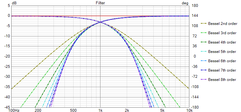
Note! This type is the target in Optimizer window when Bessel slope is selected, regardless of DSP system selection in Options.
Phase at given corner frequency (f) is -45 degrees x filter order.
Level at corner frequency (f) varies depending on slope order.
Difference between 2nd and 8th order is ca. 8.5 dB.
DSP systems using this specification: Behringer, Danville, Generic, Hypex, Marani, miniDSP, Platin, Xilica.
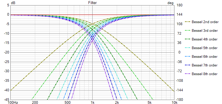
Note! This type is not supported as a target in Optimizer window.
Level at given corner frequency (f) is ca. 3 dB from max/min gain (A).
DSP systems using this specification: Analog, Behringer, FourAudio, Nova, t.racks.
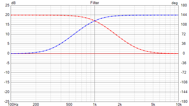
Level at given corner frequency (f) is half in dB from max/min gain (A).
DSP systems using this specification: Danville, dbx, Generic, Hypex, LEA, Marani, miniDSP, Platin, RAM, t.amp, Xilica.
Note! LEA's actual Q-factor is 0.75 x standard Q.
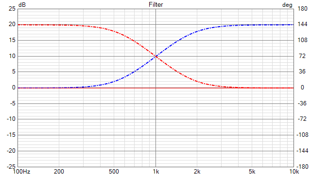
Usually has the same specification for corner frequency than 2nd order shelf. Exception is LEA having analog-compliant 1st order shelf while 2nd order shelf is digital-compliant.
Bandwidth of peak/notch equal to given Q-factor locates at ca. 3 dB from max/min gain (A).
DSP systems using this specification: Analog, Behringer, dbx, FourAudio, Hypex, LEA, Marani, Nova, t.racks, RAM, Xilica.
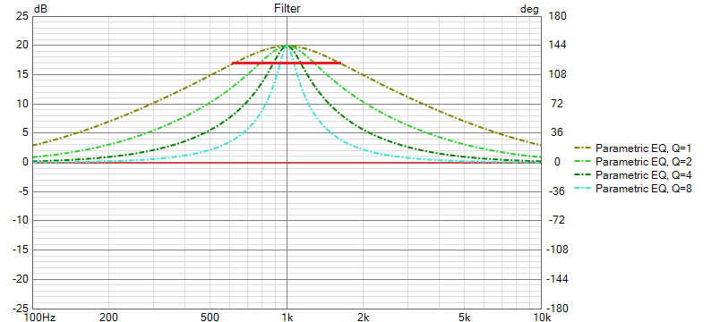
Bandwidth of peak/notch equal to given Q-factor locates at half in dB from max/min gain (A).
DSP systems using this specification: Danville, Generic, miniDSP, Platin, t.amp.